W1-W5. Integral Calculus

1. Theory

1.1 Differential of a Function

Before diving into integration, we must understand the concept of a differential. Think back to derivatives: when we write , we’re describing the rate of change of with respect to . But what are and individually?

Intuitive Understanding: Imagine you move a tiny distance along the -axis. The differential tells you approximately how much the function value changes. For a linear function like , moving units in causes units of change in . For non-linear functions, gives the best linear approximation of the actual change.

Formal Definition: If is a differentiable function on an interval , then the relationship between the derivative and the differential is given by:

We call the differential of . The differential represents an infinitesimal change in the function value corresponding to an infinitesimal change in the independent variable.

Why This Matters for Integration: The notation literally means “sum up (integrate) all the infinitesimal changes as varies.” Understanding differentials helps us see why substitution works and makes the notation more meaningful.

1.1.1 Properties of Differentials

Differentials satisfy several important algebraic properties that mirror the rules of differentiation:

1. for any constant
3. (Product Rule)
4. where (Quotient Rule)
5. (Chain Rule)

For example, and .

1.2 Antiderivatives and Indefinite Integrals

1.2.1 The Inverse Problem of Differentiation

Differentiation asks: given a function , what is its derivative ? Integration addresses the inverse problem: given a function , find a function whose derivative equals .

Real-World Motivation: Suppose you know your car’s velocity at every moment, but you want to find your position . Since velocity is the derivative of position (), you need to “undo” differentiation—this is integration! If mph (constant), then , where depends on where you started.

Another Example: If you know the rate at which water flows into a tank ( gallons per minute), integration tells you the total amount of water in the tank at any time.

Formally, let be a continuous function defined on a non-empty interval . We seek a function such that:

This function is called an antiderivative of .

1.2.2 Definition of Antiderivative

A function is called an antiderivative (or primitive function) of if and only if is differentiable on and:

For example:

• is an antiderivative of on
• is an antiderivative of on

1.2.3 Uniqueness of Antiderivatives

A fundamental theorem states: For every continuous function defined on an interval , there exists an antiderivative . Moreover, any two antiderivatives of differ by at most a constant. That is, if and are both antiderivatives of , then for some constant .

Why Constants? Think about it: if , then as well! Adding any constant doesn’t change the derivative. Conversely, if two functions have the same derivative everywhere, they can only differ by a constant—like two parallel roads that never intersect but maintain the same direction (slope) at every point.

Example: Both and are antiderivatives of , because:

1.2.4 Definition of Indefinite Integral

Let be an antiderivative of on interval . The expression , where is an arbitrary constant, is called the indefinite integral of on . We denote it by:

Here:

• is the integral sign
• is the integrand
• indicates integration with respect to
• is the constant of integration

The indefinite integral represents a family of curves, each differing by a vertical translation. Geometrically, all antiderivatives of are parallel curves in the coordinate plane.

1.3 Basic Properties of Indefinite Integrals

Let be a continuous (integrable) function, and be an arbitrary constant. Then:

1. — differentiation undoes integration
2. — taking the differential of an integral returns the integrand
3. — integration undoes differentiation
4. — linearity (sum rule)
5. for all — constant multiple rule

Note: Property (5) does not hold when because (any constant), not necessarily zero.

1.4 Basic Integration Rules

These are the fundamental formulas derived from reversing differentiation rules:

1. where
2. where
   • More generally:
3. where
   • More generally: where
4. where
12. where
    • Special case:
13. where
14. where
15. where

1.4.1 Important Remark on Elementary Functions

Not every continuous function has an antiderivative expressible in terms of elementary functions (polynomials, exponentials, logarithms, trigonometric functions, and their compositions). Examples of functions whose integrals cannot be expressed in elementary form include:

These integrals are studied as special functions (like the error function, sine integral, etc.).

1.5 Integration by Substitution (Change of Variable)

1.5.1 The Substitution Method

The substitution method is a powerful technique for evaluating integrals of the form . It works by transforming a complicated integral into a simpler one through a change of variable.

Procedure:

1. Substitute and compute
2. Rewrite the integral as
3. Integrate with respect to
4. Replace by in the final answer

Theorem (Substitution Rule): If is a differentiable function whose range is an interval , and is continuous on , then:

where and .

1.5.2 When to Use Substitution

The Key Insight: Substitution works when you can identify a “function inside a function” (composition) along with its derivative. The magic happens when the derivative of the inner function is already present (or nearly present) in the integrand!

Pattern Recognition: Look for integrals where:

• The integrand is a composite function multiplied by a factor resembling
• A substitution simplifies the integrand significantly
• The integrand contains expressions like , , , etc.

Example with Explanation: Consider .

• We see which is a function of
• Notice that the derivative of is , and we have an in the integrand!
• Substitute , so , which means

The “Chain Rule in Reverse”: Substitution undoes the chain rule. If you remember that , then integrating gives back !

1.5.3 Hermite-Ostrogradski Method

For rational functions where direct substitution is inefficient, the Hermite-Ostrogradski method separates the integral into a rational part (computed algebraically) and a logarithmic part (requiring partial fractions).

For where has repeated roots, write:

where is the GCD of and , and has only simple roots.

1.6 Integration by Parts

1.6.1 The Integration by Parts Formula

The integration by parts formula is the integral analogue of the product rule for differentiation. It states:

Equivalently:

Where Does This Come From? Remember the product rule: . Integrate both sides: Rearranging gives us integration by parts!

The Big Picture: This technique trades one integral for another. If we can’t integrate directly, we try to make easier. The art is choosing and wisely.

When to Use:

• The integrand is a product of two functions
• One function becomes simpler when differentiated (choose this as )
• The other function is easy to integrate (choose this as )

LIATE Rule (A Helpful Mnemonic): When choosing , prefer functions in this order:

1. Logarithmic functions ()
2. Inverse trig functions (, )
3. Algebraic functions (polynomials like , )
4. Trigonometric functions (, )
5. Exponential functions (, )

The function that appears first in this list should usually be (it gets simpler when differentiated).

1.6.2 Common Integration by Parts Patterns

Certain types of integrals consistently require integration by parts:

1. Logarithms: ,
   • Choose ,
2. Inverse trigonometric functions: ,
   • Choose or ,
3. Polynomial times exponential:
   • Choose ,
   • May require multiple applications
4. Polynomial times trigonometric: ,
   • Choose , or
5. Exponential times trigonometric: ,
   • Apply integration by parts twice, then solve for the integral

1.6.3 Reduction (Recurrence) Formulas

For families of integrals like or , we can derive recurrence relations that express in terms of or .

Example: Power-Exponential Integrals For :

Example: Sine Powers For :

1.7 Integration of Rational Functions

1.7.1 Partial Fraction Decomposition

A rational function is a ratio of two polynomials: where has degree and has degree .

The Challenge: Integrating complex fractions like seems hard. But what if we could split it into simpler pieces?

The Key Insight: Just as , we can often split a complex fraction into simpler ones! For example: Similarly:

The simpler fractions are easy to integrate: .

Case 1: Improper Rational Functions () If the top is “bigger” than the bottom (degree-wise), first do polynomial long division, like dividing numbers:

where is a polynomial (easy to integrate!) and (now proper).

Case 2: Proper Rational Functions () If and are coprime, decompose into partial fractions based on the factorization of :

• Linear factors: For each factor , include terms:
• Irreducible quadratic factors: For each factor with , include:

After decomposition, integrate each term separately.

1.7.2 Integration Formulas for Partial Fractions

• for
• For , complete the square and use arctangent or logarithm formulas

1.8 Integration of Trigonometric Functions

1.8.1 Common Strategies

1. Products of sines and cosines:
   • If appears to an odd power, substitute
   • If appears to an odd power, substitute
   • If both have even powers, use power-reduction formulas:
2. Products , , :
   • Use product-to-sum identities:
3. Powers of tangent and secant:
   • Use identities and
   • For , separate and use
4. Universal trigonometric substitution:
   • For (rational function of and ), use:

1.9 Integration of Hyperbolic Functions

Hyperbolic functions integrate similarly to trigonometric functions, using identities:

• ,
• ,

Substitutions like (when appears) or (when appears) are effective.

1.10 Integration of Radical Functions

1.10.1 Trigonometric Substitutions

For integrals involving radicals, trigonometric or hyperbolic substitutions often simplify the expression:

1. For : Use or
   • Then (or )
2. For : Use or
   • Then (or )
3. For : Use or
   • Then (or )

1.10.2 Rational Substitutions

For integrals of the form , substitute .

For , first complete the square, then use appropriate trigonometric substitution.

1.11 Riemann Sums and Definite Integrals

1.11.1 Motivation: Computing Area

The definite integral arises from the problem of computing the area under a curve. This is a surprisingly difficult problem that stumped mathematicians for centuries!

The Problem: Suppose we want to find the area bounded by the graph of a continuous function , the -axis, and vertical lines and . For simple shapes (rectangles, triangles), we have formulas. But what about the area under from to ?

Riemann Sums Visualization

Riemann’s Brilliant Idea: Approximate the curved region with rectangles, which we can measure! The key insight is:

1. Divide into subintervals (say, all equal width )
2. In each subinterval, construct a rectangle whose height is determined by the function value at some point
3. Sum the areas of all rectangles: Area
4. Take the limit as (rectangles become infinitesimally thin): Area

Intuition: As we use more rectangles (larger ), the approximation gets better and better. In the limit, the sum of rectangular areas becomes the exact area under the curve.

From Discrete to Continuous: The sum becomes an integral , the discrete width becomes the infinitesimal , and we get:

1.11.2 Riemann Sums

Definition: Let be a bounded function on . A partition of is a finite set of points:

The norm (or mesh) of partition is:

For each subinterval , choose a sample point . The Riemann sum associated with partition and sample points is:

1.11.3 Definition of the Definite Integral

Definition: A function is Riemann integrable on if there exists a number such that for every , there exists such that:

for all partitions with and any choice of sample points. We write:

The number is called the definite integral of from to .

Notation:

• is the lower limit of integration
• is the upper limit of integration
• is the integrand
• is the variable of integration (a dummy variable)

1.11.4 Integrable Functions

Theorem: If is continuous on , then is Riemann integrable on .

Theorem: If is bounded on and has at most finitely many discontinuities, then is Riemann integrable on .

Non-integrable Example: The Dirichlet function:

is not Riemann integrable on any interval because it is discontinuous everywhere.

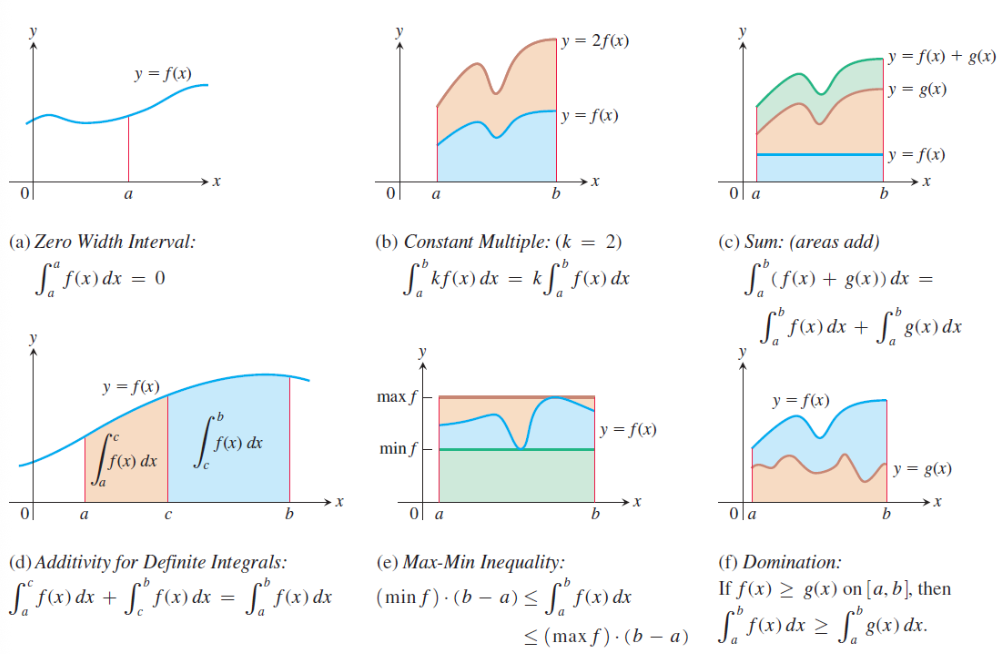
1.12 Properties of Definite Integrals

Let and be integrable functions on , and let be a constant.

1. Linearity:
2. Additivity over intervals:
3. Reversal of limits:
4. Zero-width interval:
5. Comparison property: If for all , then:
6. Absolute value inequality:
7. Max-Min inequality: If for all , then:

1.12.1 Mean Value Theorem for Definite Integrals

Theorem (Mean Value Theorem for Integrals): If is continuous on , then there exists a point such that:

The value is called the average value of on :

1.13 The Fundamental Theorem of Calculus

Why “Fundamental”? This theorem is called “fundamental” because it reveals a shocking connection: differentiation and integration are inverse operations! It’s one of the most important theorems in all of calculus.

1.13.1 Part 1: Integration as Antidifferentiation

Theorem (Fundamental Theorem of Calculus, Part 1): If is continuous on , then the function defined by:

is continuous on , differentiable on , and:

Intuitive Interpretation: Imagine represents the rate of water flowing into a tank at time . Then represents the total accumulated water from time to time .

What does mean? It’s the rate at which the accumulated amount is changing—which is exactly the flow rate at that moment, ! Differentiation undoes integration.

Key Insight: This theorem tells us that every continuous function has an antiderivative, obtained by integrating from a fixed point. The process of “accumulating” the function (integration) creates a function whose rate of change (derivative) is the original function.

More General Form: For :

1.13.2 Part 2: The Evaluation Theorem

Theorem (Fundamental Theorem of Calculus, Part 2): If is continuous on and is any antiderivative of on , then:

Notation: We often write or .

Why This is Amazing: Remember that computing directly requires taking the limit of Riemann sums—a potentially complicated process. But FTC Part 2 says: just find any antiderivative and plug in the endpoints! No limits, no sums, just simple evaluation.

Interpretation: To evaluate a definite integral, we:

1. Find any antiderivative of the integrand
2. Evaluate at the upper limit and lower limit
3. Subtract:

The Bridge: This bridges the gap between indefinite integrals (antiderivatives) and definite integrals (area/accumulation). The seemingly separate concepts—rates of change (derivatives) and accumulation (integrals)—are deeply connected.

Example: To find the area under from to :

1. Find antiderivative:
2. Evaluate:

No messy limits needed!

1.14 The Substitution Rule for Definite Integrals

Theorem (Substitution Rule for Definite Integrals): If is a continuously differentiable function on and is continuous on the range of , then:

Procedure:

1. Substitute ,
2. Change the limits: when , ; when ,
3. Integrate with respect to
4. No need to substitute back!

1.14.1 Definite Integrals of Symmetric Functions

Theorem: If is continuous on , then:

1. Even function ():
2. Odd function ():

These properties can significantly simplify calculations.

1.15 Applications of Definite Integrals

Definite integrals are incredibly powerful—they let us compute areas, volumes, lengths, and many other quantities. The key idea is always the same: slice, approximate, sum, and take the limit.

1.15.1 Area Between Curves

The Idea: To find the area between two curves, imagine slicing the region into thin vertical strips. Each strip has:

• Width: (infinitesimal)
• Height: (difference between upper and lower curves)
• Area of one strip:

Summing all strips gives the total area:

Important: If the curves intersect, split the integral at intersection points and ensure the upper function is always subtracted from the lower (sometimes this switches!).

Area Between Curves: sin and cos

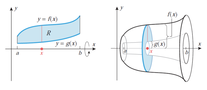
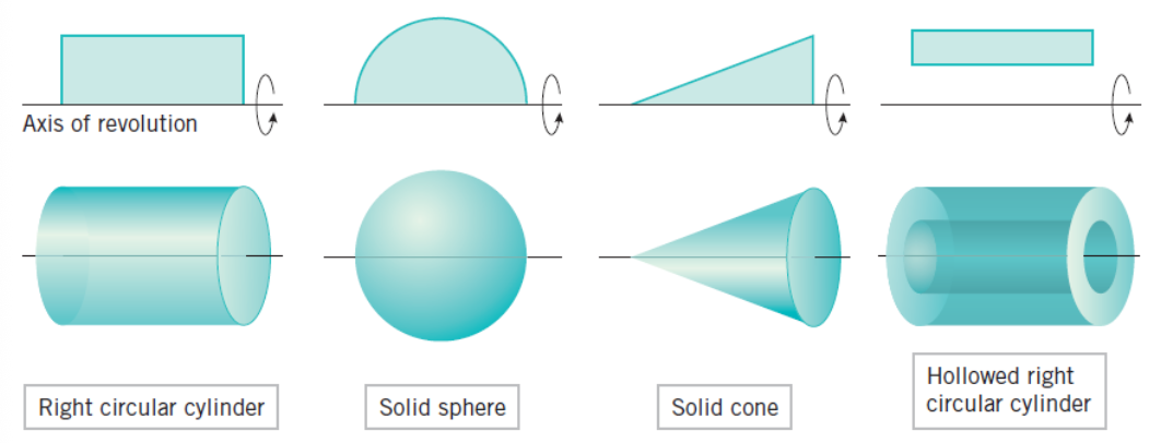
1.15.2 Volume of Solids of Revolution

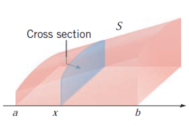
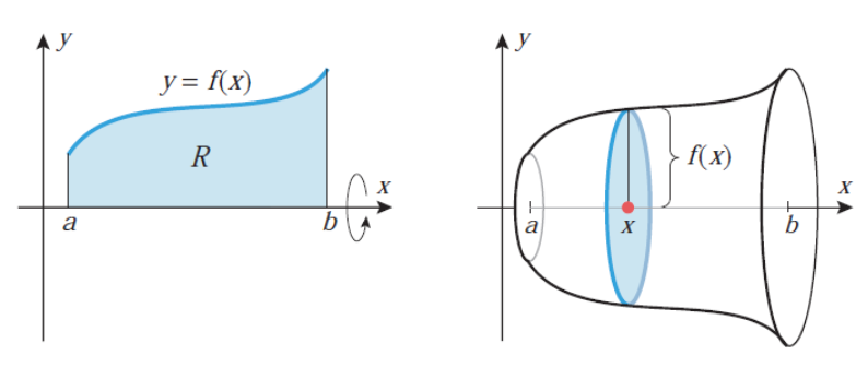
When we rotate a region around an axis, we create a 3D solid. How do we find its volume?

Disk Method: Imagine slicing the solid perpendicular to the axis of rotation. Each slice is approximately a circular disk!

• Radius of disk:
• Thickness:
• Volume of one disk: (area of circle times thickness)

Summing all disks from to :

Cross Section of Solid

Disk Method and Volume Under Curve

Washer Method: If there’s a hole in the middle (region between two curves), each slice is a washer (disk with a hole):

• Outer radius: , Inner radius:
• Area of washer:
• Volume:

Disk and Washer Methods

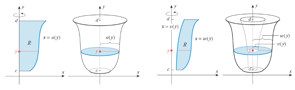
Shell Method: When revolving about the -axis, imagine the solid as nested cylindrical shells:

• Radius of shell:
• Height:
• Circumference:
• “Surface area” of shell:
• Thickness:
• Volume:

Shell Method and Solids of Revolution

Alternative Solids of Revolution

1.15.3 Arc Length

The Challenge: How do we measure the length of a curve? For a straight line, it’s easy. For a curve, we need calculus!

The Idea: Approximate the curve with tiny straight line segments, measure each segment, sum them up, and take the limit.

Consider a tiny piece of the curve from to . Using the Pythagorean theorem:

• Horizontal change:
• Vertical change:
• Length of tiny segment:

Summing all segments gives the total length:

For Parametric Curves: If the curve is given by , the same idea applies:

• At time , the position is
• A tiny time interval causes changes and
• Segment length:

1.15.4 Surface Area of Revolution

If the curve from to is revolved about the -axis, the surface area is:

1.16 Improper Integrals

1.16.1 Motivation

The definite integral is defined for finite intervals and bounded, integrable functions. But real-world problems often involve infinity!

Real-World Questions:

• What’s the total energy radiated by the sun over all future time? (Infinite interval)
• How much work is needed to escape Earth’s gravitational pull? (Infinite distance)
• What’s the probability that a randomly chosen number from a bell curve exceeds 1000? (Integral over infinite range)

The Challenge: We can’t directly compute “infinite sums.” We need a careful limiting process.

Improper integrals extend the concept of integration to:

1. Infinite intervals: , , or
2. Unbounded integrands: Functions with vertical asymptotes in (like near )

Key Question: Does the integral have a finite value (converges) or not (diverges)?

1.16.2 Type 1: Infinite Intervals

Definition: If is continuous on , we define:

If the limit exists (is finite), the integral converges to that value. Otherwise, it diverges.

Similarly:

For the entire real line:

Both integrals on the right must converge for the left side to converge.

1.16.3 Type 2: Discontinuous Integrands

If has a discontinuity at (right endpoint):

If has a discontinuity at (left endpoint):

If has a discontinuity at :

Both integrals on the right must converge.

1.16.4 Tests for Convergence

When we cannot evaluate an improper integral directly, we use comparison tests. The idea is simple: compare your integral with one you already understand.

The Intuition: If a smaller function has infinite area, so does a larger one. Conversely, if a larger function has finite area, so does a smaller one. It’s like comparing two people’s bank accounts: if the person who earns less has saved , the person who earns more definitely has at least that much!

Direct Comparison Test: Let and be continuous on with for all (think: “ is smaller than ”).

1. If converges (the bigger area is finite), then converges (the smaller area must also be finite)
2. If diverges (the smaller area is infinite), then diverges (the bigger area must also be infinite)

Strategy: Compare your integral with standard functions whose convergence you know (see below).

Limit Comparison Test: If and are continuous on , and:

Then:

1. If , both and either both converge or both diverge
2. If and converges, then converges
3. If and diverges, then diverges

Common Comparison Functions:

• converges if , diverges if
• converges

1.16.5 Cauchy Integral Test for Series

Theorem: Let be a series with non-negative terms, and let be a continuous, decreasing function on such that . Then the series and the integral are of the same nature (both converge or both diverge).

This provides a powerful link between improper integrals and infinite series.

---

2. Definitions

• Differential: For a differentiable function , the differential is , representing an infinitesimal change in the function value.
• Antiderivative (Primitive Function): A function is an antiderivative of on interval if for all .
• Indefinite Integral: The expression representing the general form of all antiderivatives of , where is an arbitrary constant.
• Integrand: The function being integrated in .
• Constant of Integration: The arbitrary constant appearing in indefinite integrals, accounting for the fact that antiderivatives differ by constants.
• Integration by Substitution: A technique for evaluating integrals by changing the variable of integration using and .
• Integration by Parts: A technique based on the product rule, given by .
• Rational Function: A function of the form where and are polynomials.
• Partial Fraction Decomposition: The process of expressing a rational function as a sum of simpler fractions with linear or irreducible quadratic denominators.
• Proper Rational Function: A rational function where the degree of the numerator is less than the degree of the denominator .
• Improper Rational Function: A rational function where the degree of the numerator is greater than or equal to the degree of the denominator.
• Reduction (Recurrence) Formula: A formula expressing an integral in terms of simpler integrals , , etc.
• Partition: A finite set of points dividing an interval into subintervals, where .
• Norm (Mesh) of a Partition: The maximum width of subintervals in a partition, .
• Riemann Sum: An approximation of an integral given by , where are sample points and .
• Definite Integral: The limit of Riemann sums as the partition norm approaches zero, denoted , representing the signed area under the curve or the accumulation of from to .
• Riemann Integrable: A function is Riemann integrable on if the limit defining the definite integral exists.
• Lower Limit of Integration: The value in .
• Upper Limit of Integration: The value in .
• Average Value of a Function: For a continuous function on , the average value is .
• Fundamental Theorem of Calculus, Part 1: States that if , then .
• Fundamental Theorem of Calculus, Part 2 (Evaluation Theorem): States that where is any antiderivative of .
• Even Function: A function satisfying for all in its domain.
• Odd Function: A function satisfying for all in its domain.
• Solid of Revolution: A three-dimensional solid obtained by rotating a two-dimensional region about an axis.
• Disk Method: A technique for computing volumes of solids of revolution using circular cross-sections perpendicular to the axis of rotation.
• Washer Method: A variation of the disk method for regions between two curves, using annular (ring-shaped) cross-sections.
• Shell Method: A technique for computing volumes using cylindrical shells parallel to the axis of rotation.
• Arc Length: The distance along a curve, computed by integrating for a curve .
• Surface Area of Revolution: The area of the surface obtained by revolving a curve about an axis.
• Improper Integral: An integral with infinite limits of integration or an unbounded integrand, defined as a limit of proper integrals.
• Convergent Improper Integral: An improper integral whose defining limit exists and is finite.
• Divergent Improper Integral: An improper integral whose defining limit does not exist or is infinite.
• Direct Comparison Test: A test for convergence of improper integrals based on comparing with a function of known convergence behavior.
• Limit Comparison Test: A test for convergence based on the limit of the ratio of two functions as .
• Cauchy Integral Test: A test relating the convergence of an infinite series to the convergence of where .

---

3. Formulas

Basic Integration Rules:

• Constant:
• Power Rule: (for )
• General Power Rule: (for )
• Reciprocal: (for )
• General Logarithm:
• Exponential (base e): (for )
• General Exponential: (for )

Trigonometric Integrals:

• Sine:
• Cosine:
• Secant Squared:
• Cosecant Squared:
• Secant Tangent:
• Cosecant Cotangent:
• Tangent:
• Cotangent:
• Secant:
• Cosecant:

Hyperbolic Integrals:

• Hyperbolic Sine:
• Hyperbolic Cosine:
• Hyperbolic Secant Squared:
• Hyperbolic Cosecant Squared:
• Hyperbolic Tangent:
• Hyperbolic Cotangent:

Inverse Trigonometric Integrals:

• Arctangent Form: (for )
• Arcsine Form: (for )
• Inverse Hyperbolic Sine:
• Inverse Hyperbolic Cosine: (for )
• General Form 1:

Integration by Parts Formula:

Substitution Rule for Definite Integrals:

Fundamental Theorem of Calculus:

• Part 1:
• Part 2: where
• Leibniz Rule:

Symmetry Properties for Definite Integrals:

• Even Function: (if )
• Odd Function: (if )

Applications of Definite Integrals:

• Area Between Curves: (where )
• Volume by Disk Method:
• Volume by Washer Method: (where )
• Volume by Shell Method: (revolving about -axis)
• Arc Length:
• Parametric Arc Length:
• Surface Area of Revolution: (about -axis)
• Average Value:

Improper Integrals:

• Type 1 (Infinite Interval):
• Type 2 (Discontinuity at ):
• -Integral Test: converges if , diverges if

Trigonometric Identities (for Integration):

• Power Reduction: ,
• Product-to-Sum:
• Product-to-Sum:
• Product-to-Sum:
• Pythagorean:
• Universal Substitution: gives , ,

Hyperbolic Identities (for Integration):

• Power Reduction: ,
• Pythagorean:
• Pythagorean:

---

4. Practice

4.1. Compute (Lab 1, Warm-Up 1)

Compute the integral using basic integration rules.

Click to see the solution

Key Concept: Apply the power rule and linearity of integration.

1. Split the integral:
2. Integrate each term:
3. Simplify:

Answer:

4.2. Compute (Lab 1, Integration by Parts 2)

Evaluate using integration by parts (may require multiple applications).

Click to see the solution

Key Concept: When integrating polynomial times exponential, choose as the polynomial.

1. First application of integration by parts:
   • Let , so
   • Let , so
2. Second application for :
   • Let , so
   • Let , so
3. Substitute back:
4. Simplify:

Answer:

4.3. Compute (Lab 1, Integration by Parts 3)

Evaluate using integration by parts.

Click to see the solution

Key Concept: For integrals of inverse trigonometric functions alone, use = inverse trig function, .

1. Set up integration by parts:
   • Let , so
   • Let , so
2. Apply the formula:
3. Evaluate the remaining integral using substitution: Let , so
4. Substitute back:

Answer:

4.4. Compute (Lab 1, Integration by Parts 4)

Evaluate using integration by parts.

Click to see the solution

1. Set up integration by parts:
   • Let , so
   • Let , so
2. Apply the formula:
3. Integrate:

Answer:

4.5. Compute (Lab 1, Integration by Parts 5, Advanced)

Derive a reduction formula.

Click to see the solution

Key Concept: Use integration by parts to derive a recurrence relation.

1. Rewrite the integral:
2. Set up integration by parts:
   • Let , so
   • Let , so
3. Apply the formula:
4. Use :
5. Solve for the original integral:
6. Derive the reduction formula:

Answer (Reduction Formula):

4.6. Compute (Lab 1, Homework 1)

Evaluate using integration by parts.

Click to see the solution

1. Set up integration by parts:
   • Let , so
   • Let , so
2. Apply the formula:
3. Integrate:

Answer:

4.7. Compute (Lab 1, Homework 3)

Evaluate using substitution.

Click to see the solution

1. Choose substitution: Let , so , which means
2. Substitute:
3. This requires another substitution or trigonometric substitution. Alternatively, recognize that:

Answer:

4.8. Compute (Lab 1, Homework 5)

Evaluate using trigonometric substitution.

Click to see the solution

Key Concept: For , use or .

1. Choose substitution: Let , so
   • Then
2. Substitute:
3. Simplify using identities:
4. Use power-reduction formula:
5. Express in terms of : From , we have and
   • ,
6. Final answer:

Answer: (or equivalent form)

4.9. Compute (Lab 1, Warm-Up 2)

Compute the integral using basic integration rules.

Click to see the solution

1. Split the integral:
2. Apply exponential and trigonometric integration rules:

Answer:

4.10. Compute (Lab 1, Warm-Up 3)

Compute the integral.

Click to see the solution

1. Rewrite using exponent notation:
2. Apply the power rule:
3. Simplify:

Answer:

4.11. Compute (Lab 1, Substitution 1)

Evaluate using the substitution method.

Click to see the solution

Key Concept: Use substitution when the integrand contains a function and its derivative.

1. Choose substitution: Let
2. Compute differential: , so
3. Substitute:
4. Integrate:
5. Substitute back:

Answer:

4.12. Compute (Lab 1, Substitution 2)

Evaluate using substitution.

Click to see the solution

1. Choose substitution: Let
2. Compute differential:
3. Substitute:
4. Integrate:
5. Substitute back:

Answer:

4.13. Compute (Lab 1, Substitution 3)

Evaluate using substitution.

Click to see the solution

1. Choose substitution: Let
2. Compute differential: , so
3. Substitute:
4. Integrate:
5. Substitute back:

Answer:

4.14. Compute (Lab 1, Substitution 4)

Evaluate using substitution.

Click to see the solution

1. Choose substitution: Let
2. Compute differential:
3. Substitute:
4. Integrate:
5. Substitute back:

Answer:

4.15. Compute (Lab 1, Substitution 5)

Evaluate using substitution (requires algebraic manipulation).

Click to see the solution

Key Concept: When substitution leaves in the integrand, express in terms of .

1. Choose substitution: Let , so
2. Compute differential: , so
3. Substitute:
4. Expand:
5. Integrate:
6. Simplify and substitute back:

Answer:

4.16. Compute (Lab 1, Integration by Parts 1)

Evaluate using integration by parts.

Click to see the solution

Key Concept: Choose (logarithm simplifies when differentiated) and (polynomial easy to integrate).

1. Set up integration by parts:
   • Let , so
   • Let , so
2. Apply the formula:
3. Simplify the remaining integral:
4. Perform polynomial long division:
5. Integrate:
6. Simplify:

Answer:

4.17. Compute (Lab 2, Rational Functions 1)

Evaluate using partial fraction decomposition.

Click to see the solution

Key Concept: Factor the denominator and decompose into partial fractions.

1. Factor the denominator:
2. Set up partial fractions:
3. Solve for and : Multiply both sides by :
   • Set :
   • Set :
4. Integrate:

Answer:

4.18. Compute (Lab 2, Rational Functions 2)

Evaluate using partial fractions with repeated irreducible quadratic factors.

Click to see the solution

Key Concept: For repeated irreducible quadratic factors, include terms for each power.

1. Set up partial fractions:

2. Multiply both sides by :

3. Expand and collect terms:

4. Match coefficients:

   • :
   • :
   • :
   • :

5. Integrate:

   For the first integral, let :

   For the second integral:

   • First part (substitution ):

   • Second part (arctangent form with reduction): requires reduction formula or trigonometric substitution

     Using :

6. Combine results:

Answer:

4.19. Compute (Lab 2, Rational Functions 3)

Evaluate using partial fractions with repeated linear factors.

Click to see the solution

1. Set up partial fractions:
2. Multiply by :
3. Solve for constants:
   • Set :
   • Set :
   • Set :
4. Integrate:

Answer:

4.20. Compute (Lab 2, Rational Functions 4)

Evaluate an improper rational function.

Click to see the solution

Key Concept: When degree of numerator degree of denominator, perform polynomial long division first.

1. Polynomial long division:
2. Decompose the proper fraction:
   • Set :
   • Set :
3. Integrate:

Answer:

4.21. Compute (Lab 2, Trigonometric 1)

Evaluate using substitution.

Click to see the solution

1. Choose substitution: Let , so
2. Substitute:
3. Integrate:

Answer:

4.22. Compute (Lab 2, Trigonometric 2)

Evaluate using substitution.

Click to see the solution

1. Choose substitution: Let , so
2. Substitute:
3. Substitute back:

Answer:

4.23. Compute (Lab 2, Trigonometric 3)

Evaluate using product-to-sum identities.

Click to see the solution

Key Concept: Use .

1. Apply identity:
2. Integrate:

Answer:

4.24. Compute (Lab 2, Trigonometric 4)

Evaluate using the identity .

Click to see the solution

1. Rewrite using identity:
2. Split the integral:
3. Evaluate each part:
   • For , let , :
   • For , let :
4. Combine:

Answer:

4.25. Compute (Lab 2, Hyperbolic 1)

Evaluate using hyperbolic identities and substitution.

Click to see the solution

Key Concept: Use the identity or product-to-sum formulas.

1. Apply identity:
2. Choose substitution: Let , so
3. Substitute:
4. Integrate:
5. Substitute back:

Answer:

4.26. Compute (Lab 2, Hyperbolic 2)

Evaluate using substitution.

Click to see the solution

1. Choose substitution: Let , so

2. Substitute:

3. Integrate:

4. Substitute back:

   (Since for all , the absolute value is not needed)

Answer:

4.27. Compute (Lab 2, Hyperbolic 3)

Evaluate using the identity .

Click to see the solution

1. Apply identity:
2. Integrate:

Answer:

4.28. Compute (Lab 2, Radical Functions 1)

Evaluate using substitution.

Click to see the solution

1. Choose substitution: Let , so , which means
2. Substitute:
3. Integrate:
4. Substitute back:

Answer:

4.29. Compute (Lab 2, Radical Functions 2)

Evaluate using substitution and algebraic manipulation.

Click to see the solution

Key Concept: Rewrite to separate simpler integrals.

1. Rewrite the integrand:

2. Alternative approach - substitution: Let , so

   • Then

3. Simplify using identities:

4. This requires advanced techniques. Alternative: Use integration by parts or table of integrals.

   Result:

Answer:

4.30. (Lab 3, Hyperbolic Functions Integration, Basic)

Evaluate the indefinite integral of .

Click to see the solution

Key Concept: Use the hyperbolic identity , which allows us to rewrite in terms of a function whose integral is known.

1. Apply the hyperbolic identity: We know that
2. Rewrite the integral:
3. Use the linearity of integration:
4. Integrate each term:
   • (standard integral)
5. Combine the results:

Answer:

4.31. (Lab 3, Hyperbolic Functions Integration, Basic)

Evaluate the indefinite integral of .

Click to see the solution

Key Concept: Use the double angle formula to simplify the integrand into a form that allows substitution.

1. Apply the double angle identity:
2. Rewrite the integral:
3. Apply substitution: Let , so
4. Transform the integral:
5. Integrate with respect to :
6. Substitute back: Replace :

Answer:

4.32. (Lab 3, Hyperbolic Functions Integration, Basic)

Evaluate the indefinite integral of .

Click to see the solution

Key Concept: Recognize that the derivative of the denominator is , which is exactly the numerator. This is a perfect candidate for substitution.

1. Identify the substitution: Let , so
2. Transform the integral:
3. Integrate:
4. Substitute back: Replace :
5. Simplify: Since for all , we have , so we can drop the absolute value:

Answer:

4.33. (Lab 3, Trigonometric Functions Integration, Basic)

Evaluate the indefinite integral of .

Click to see the solution

Key Concept: The integrand contains raised to an odd power and to the first power. Since the derivative of is , we use substitution with .

1. Identify the substitution: Let , so
2. Transform the integral:
3. Integrate using the power rule:
4. Substitute back: Replace :

Answer:

4.34. (Lab 3, Trigonometric Functions Integration, Basic)

Evaluate the indefinite integral of .

Click to see the solution

Key Concept: The numerator is the derivative of the negative of the denominator’s inner function. Specifically, . We can use substitution with .

1. Identify the substitution: Let , so , which means
2. Transform the integral:
3. Integrate:
4. Substitute back: Replace :
5. Simplify: Since , we have , so . We can drop the absolute value:

Answer:

4.35. (Lab 3, Trigonometric Functions Integration, Intermediate)

Evaluate the indefinite integral of .

Click to see the solution

Key Concept: For powers of tangent, we use the identity to decompose the odd power into a manageable form.

1. Decompose using the identity: , so:

2. Rewrite the integral:

3. Evaluate the first integral: Let , so

4. Evaluate the second integral: We can write

   Let , so :

   This can also be written as

5. Combine the results:

Answer: (or equivalently: )

4.36. (Lab 3, Trigonometric Functions Integration, Intermediate)

Evaluate the indefinite integral of .

Click to see the solution

Key Concept: For products of sines and cosines with different arguments, use the product-to-sum identity: .

1. Apply the product-to-sum identity: With and :
2. Simplify using :
3. Rewrite the integral:
4. Integrate each term:
5. Combine the results:

Answer:

4.37. (Lab 3, Trigonometric Functions Integration, Advanced)

Evaluate the indefinite integral of using trigonometric substitution.

Click to see the solution

Key Concept: For integrals involving , use the trigonometric substitution . This transforms the radical into a trigonometric function that simplifies the integrand significantly.

1. Set up the trigonometric substitution: Let , so

2. Simplify the radical: (We use since for the principal branch)

3. Transform the integral:

4. Rewrite using trigonometric functions:

5. Using the result from advanced integration techniques: The integral evaluates to .

6. Express in terms of original variable: From :

   • and
   • and

Answer:

4.38. (Lab 3, Rational Functions, Advanced)

Evaluate the indefinite integral of using partial fraction decomposition.

Click to see the solution

Key Concept: For rational functions with irreducible quadratic factors in the denominator, we decompose the numerator strategically to separate terms with the derivative of the denominator factor from constant terms.

1. Set up the partial fraction decomposition: Since the denominator is , we decompose:

2. Multiply both sides by :

3. Expand the right side:

4. Compare coefficients:

   • Coefficient of :
   • Coefficient of :
   • Coefficient of :
   • Coefficient of :

5. Write the decomposition:

6. Integrate the first term: For , let , so :

7. Integrate the second term: Split into two parts:

   For the first part, let , so :

   For the second part, use the formula

   With , so :

8. Combine all parts:

Answer:

4.39. Riemann Sum: with (Left Endpoint) (Lab 3, Riemann Sums, Numerical Integration)

Approximate using a left Riemann sum with subintervals.

Click to see the solution

Key Concept: A Riemann sum approximates the area under a curve by dividing the interval into subintervals and using rectangles. The left endpoint method evaluates the function at the left end of each subinterval.

1. Calculate the step size:
2. Identify the partition points:
3. Evaluate the function at left endpoints:
4. Compute the left Riemann sum:
5. Compare with the exact value:
6. Compute the error:

Answer: The left Riemann sum approximation is (exact value: , error: )

4.40. Riemann Sum: with (Right Endpoint) (Lab 3, Riemann Sums, Numerical Integration)

Approximate using a right Riemann sum with subintervals.

Click to see the solution

Key Concept: The right endpoint method evaluates the function at the right end of each subinterval. This typically gives a different approximation than the left endpoint method, and for increasing functions, it tends to overestimate the area.

1. Calculate the step size:
2. Identify the partition points:
3. Evaluate the function at right endpoints:
4. Compute the right Riemann sum:
5. Compare with the exact value:
6. Compute the error:

Answer: The right Riemann sum approximation is (exact value: , error: )

4.41. Riemann Sum: with (Midpoint) (Lab 3, Riemann Sums, Numerical Integration)

Approximate using a midpoint Riemann sum with subintervals.

Click to see the solution

Key Concept: The midpoint method evaluates the function at the midpoint of each subinterval. This method typically provides better accuracy than left or right endpoint methods because it accounts for the function’s behavior more uniformly across each subinterval.

1. Calculate the step size:
2. Identify the partition points:
3. Compute midpoints of each subinterval:
   • Subinterval 1: , midpoint:
   • Subinterval 2: , midpoint:
   • Subinterval 3: , midpoint:
   • Subinterval 4: , midpoint:
4. Evaluate the function at midpoints:
5. Compute the midpoint Riemann sum:
6. Compare with the exact value:
7. Compute the error:

Answer: The midpoint Riemann sum approximation is (exact value: , error: )

4.42. Compute (Lab 3, Hyperbolic)

Evaluate using hyperbolic identity.

Click to see the solution

Key Concept: Use or .

1. Rewrite:
2. Integrate:

Answer:

4.43. Compute (Lab 3, Hyperbolic)

Evaluate using product formula.

Click to see the solution

1. Use :
2. Let :

Answer:

4.44. Compute (Lab 3, Hyperbolic)

Evaluate using substitution.

Click to see the solution

1. Let :
2. Substitute back:

Answer:

4.45. Compute (Lab 3, Trigonometric)

Evaluate using substitution.

Click to see the solution

1. Let :

Answer:

4.46. Compute (Lab 3, Trigonometric)

Evaluate using substitution.

Click to see the solution

1. Let :
2. Substitute back:

Answer:

4.47. Compute (Lab 3, Trigonometric)

Evaluate using identity and substitution.

Click to see the solution

1. Rewrite:
2. For first integral, let :
3. For second integral:
4. Combine:

Answer:

4.48. Compute (Lab 3, Trigonometric)

Evaluate using product-to-sum formula.

Click to see the solution

Key Concept: Use .

1. Apply formula:
2. Integrate:

Answer:

4.49. Compute (Lab 3, Trigonometric Substitution)

Evaluate using trigonometric substitution.

Click to see the solution

Key Concept: For , use .

1. Let , :
2. Rewrite:
3. Convert to sines and cosines:
4. Let :
5. Back-substitute: From , we have :

Answer:

4.50. Compute (Lab 3, Partial Fractions)

Evaluate using partial fractions.

Click to see the solution

Key Concept: For repeated quadratic factors, use appropriate partial fraction form.

1. Set up:
2. Multiply both sides by :
3. Expand:
4. Match coefficients:
   • :
   • :
   • :
   • :
5. Integrate:

Answer:

4.51. Compute (Riemann Sum with ) (Lab 3, Riemann Sums)

Approximate and compute using left, right, and midpoint rules.

Click to see the solution

Key Concept: Riemann sums approximate definite integrals using rectangular partitions.

1. Partition: into equal subintervals:
   • Subintervals:
   • Sample points: (left), or (right), or (midpoint)
2. Left Riemann Sum:
3. Right Riemann Sum:
4. Midpoint Riemann Sum:
5. Exact integral:

Answer: Left: , Right: , Midpoint: , Exact:

4.52. Compute (Riemann Sum with ) (Lab 3, Riemann Sums)

Approximate using different methods.

Click to see the solution

1. Partition: into equal subintervals:
   • Subintervals:
2. Left Riemann Sum:
3. Right Riemann Sum:
4. Midpoint Riemann Sum:
5. Exact integral:

Answer: Left: , Right: , Midpoint: , Exact:

4.53. Compute (Riemann Sum with ) (Lab 3, Riemann Sums)

Approximate using Riemann sums.

Click to see the solution

1. Partition: into equal subintervals:
   • Subintervals:
2. Left Riemann Sum:
3. Right Riemann Sum:
4. Midpoint Riemann Sum:
5. Exact integral:

Answer: Left: , Right: , Midpoint: , Exact:

4.54. Evaluate (Lab 4, Task 1a)

Evaluate the definite integral.

Click to see the solution

Key Concept: Use substitution to evaluate the definite integral.

1. Substitution: Let , then
2. Change limits:
   • When :
   • When :
3. Substitute:
4. Integrate:

Answer:

4.55. Evaluate (Lab 4, Task 1b)

Evaluate the definite integral.

Click to see the solution

Key Concept: Use substitution with .

1. Substitution: Let , then
2. Change limits:
   • When :
   • When :
3. Substitute:
4. Integrate:

Answer:

4.56. Evaluate (Lab 4, Task 1c)

Evaluate the definite integral.

Click to see the solution

Key Concept: Use substitution with .

1. Substitution: Let , then
2. Change limits:
   • When :
   • When :
3. Substitute:
4. Integrate:

Answer:

4.57. Evaluate (Lab 4, Task 1d)

Evaluate the definite integral.

Click to see the solution

Key Concept: Use substitution with .

1. Substitution: Let , then , so
2. Change limits:
   • When :
   • When :
3. Substitute:
4. Integrate:

Answer:

4.58. Find the area bounded by and (Lab 4, Task 2a)

Find the area between the two curves.

Click to see the solution

Key Concept: Find intersection points, then integrate the difference of the upper and lower functions.

1. Find intersection points: Set
2. Determine which function is above:
   • At : and
   • So on
3. Set up the integral:
4. Integrate:
5. Evaluate:
   • At :
   • At :

Answer: square units

4.59. Find the area bounded by and from to (Lab 4, Task 2b)

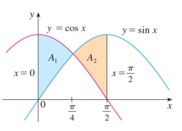
Find the area between the sine and cosine curves.

Click to see the solution

Key Concept: Determine which function is above on the given interval, then integrate the difference.

1. Determine which function is above:
   • At : and , so
   • At : (they meet)
   • So on
2. Set up the integral:
3. Integrate:
4. Evaluate:
   • At :
   • At :

Answer: square units

4.60. Find the area bounded by and from to (Lab 4, Task 2c)

Find the area between the line and the parabola.

Click to see the solution

Key Concept: The line is above the parabola on .

1. Determine which function is above:
   • At : and
   • So on (since for )
2. Set up the integral:
3. Integrate:
4. Evaluate:

Answer: square units

4.61. Find the volume generated by rotating the region bounded by , , and about the x-axis (Lab 4, Task 3)

Find the volume of revolution using the disk method.

Click to see the solution

Key Concept: Use the disk method: .

1. Identify the radius: When rotating about the x-axis,
2. Set up the integral:
3. Integrate:

Answer: cubic units

4.62. Find the volume of the solid from rotating from to about the x-axis (Lab 4, Task 4)

Find the volume of revolution using the disk method.

Click to see the solution

Key Concept: Use the disk method with .

1. Set up the integral:
2. Integrate:

Answer: cubic units

4.63. Find the volume of the solid from rotating the region between and about the x-axis (Lab 4, Task 5)

Find the volume using the washer method.

Click to see the solution

Key Concept: Use the washer method: .

1. Find intersection points: Set , so , giving or
2. Identify outer and inner radii:
   • Outer radius: (farther from x-axis)
   • Inner radius: (closer to x-axis)
3. Set up the integral:
4. Integrate:

Answer: cubic units

4.64. Find the length of from to (Lab 4, Task 6)

Find the arc length of the curve.

Click to see the solution

Key Concept: Use the arc length formula .

1. Find the derivative:
2. Calculate :
3. Set up the integral:
4. Substitute: Let , then
   • When :
   • When :
5. Integrate:

Answer: units

4.65. Find the arc length of from to (Lab 4, Task 7)

Find the arc length of the logarithmic curve.

Click to see the solution

Key Concept: Use the arc length formula and simplify using trigonometric identities.

1. Find the derivative:
2. Calculate :
3. Set up the integral: (Note: on , so )
4. Integrate:
5. Evaluate:
   • At : ,
   • At : ,

Answer: units

4.66. Compute the surface area from rotating from to about the x-axis (Lab 4, Task 8)

Find the surface area of revolution.

Click to see the solution

Key Concept: Use the surface area formula .

1. Find the derivative:
2. Calculate :
3. Set up the integral:
4. Substitute: Let , then , so
   • When :
   • When :
5. Integrate:

Answer: square units

4.67. Find the area bounded by and (Lab 4, Homework 1a)

Find the area between the parabola and the line.

Click to see the solution

Key Concept: Find intersection points and integrate the difference.

1. Find intersection points: Set
2. Determine which function is above:
   • At : and
   • So on
3. Set up the integral:
4. Integrate:
5. Evaluate:
   • At :
   • At :

Answer: square units

4.68. Find the area bounded by and (Lab 4, Homework 1b)

Find the area between the square root function and the line.

Click to see the solution

Key Concept: Find intersection points and integrate the difference.

1. Find intersection points: Set
2. Determine which function is above:
   • At : and
   • So on
3. Set up the integral:
4. Integrate:
5. Evaluate:

Answer: square units

4.69. Find the area bounded by and from to (Lab 4, Homework 1c)

Find the area between cosine and sine over a quarter period.

Click to see the solution

Key Concept: The curves intersect at , so we need two integrals.

1. Find intersection: Set , so , giving on
2. Determine which function is above:
   • On : (check at : )
   • On : (check at : )
3. Set up the integrals:
4. Integrate:
5. Evaluate first integral:
6. Evaluate second integral:
7. Total area:

Answer: square units

4.70. Find the area bounded by and (Lab 4, Homework 1d)

Find the area between two parabolas opening horizontally.

Click to see the solution

Key Concept: Integrate with respect to since the functions are given as .

1. Find intersection points: Set
2. Determine which function is to the right:
   • At : and
   • So on
3. Set up the integral:
4. Integrate:
5. Evaluate:
   • At :
   • At :

Answer: square units

4.71. Find the volume of the solid obtained by rotating the region bounded by , , and about the y-axis (Lab 4, Homework 2)

Find the volume using the shell method or disk method with respect to .

Click to see the solution

Key Concept: Use the disk method with respect to . Express in terms of : .

1. Express in terms of : Since , we have
2. Find the bounds: When , , so
3. Set up the integral (washer method): The region is bounded by on the left and on the right, so:
   • Outer radius:
   • Inner radius:
4. Integrate:

Answer: cubic units

4.72. Find the volume of the solid obtained by rotating the region bounded by , , and about the line (Lab 4, Homework 3)

Find the volume using the disk method with shifted axis.

Click to see the solution

Key Concept: When rotating about , the radius is the distance from the curve to the line .

1. Find the intersection: When , , so
2. Identify the radius: Distance from to is
3. Set up the integral:
4. Expand:
5. Integrate:
6. Evaluate:

Answer: cubic units

4.73. Find the volume when the region bounded by , , and is rotated about the x-axis (Lab 4, Homework 4)

Find the volume using the washer method.

Click to see the solution

Key Concept: The region is bounded above by and below by for .

1. Identify outer and inner radii:
   • Outer radius:
   • Inner radius:
2. Set up the integral:
3. Integrate:
4. Evaluate:

Answer: cubic units

4.74. Find the length of the curve from to (Lab 4, Homework 5)

Find the arc length of the curve.

Click to see the solution

Key Concept: Use the arc length formula and look for a perfect square under the radical.

1. Find the derivative:
2. Calculate :
3. Set up the integral:
4. Integrate:
5. Evaluate:

Answer: units

4.75. Find the surface area generated by rotating , , about the x-axis (Lab 4, Homework 6)

Find the surface area of revolution for a semicircle.

Click to see the solution

Key Concept: Recognize that is the upper half of a circle with radius 2.

1. Find the derivative:
2. Calculate :
3. Set up the integral:
4. Integrate:

Answer: square units

4.76. Find the surface area when the curve for is rotated about the x-axis (Lab 4, Homework 7)

Find the surface area of revolution.

Click to see the solution

Key Concept: Use the surface area formula and simplify using trigonometric identities.

1. Find the derivative:

2. Calculate :

3. Set up the integral:

4. Substitute: Let , then

   This substitution doesn’t directly simplify. Instead, use integration by parts:

   Let ,

   Then ,

   This becomes complex. Alternatively, use the fact that:

   (This can be verified by differentiation or found in integral tables)

5. Evaluate:

6. At :

7. At : ,

8. Final answer:

Answer: square units (or square units)

4.77. Find the volume of the wedge cut from a cylinder of radius 3 by two planes (Lab 5, Recap 1)

A curved wedge is cut from a circular cylinder of radius 3 by two planes. One plane is perpendicular to the axis, the other makes a angle at the center. Find the wedge’s volume.

Click to see the solution

Key Concept: Slice the solid with cross-sections perpendicular to the -axis. Because the cutting plane makes a angle, the height of each cross-section at position equals itself.

Set up coordinates so the cylinder has equation (axis along the -axis). The wedge is bounded below by and above by (the plane), for .

1. Find the cross-sectional area at position : For fixed , ranges from to and ranges from to . The cross-section is a rectangle with:
   • Width:
   • Height: (the height of the wedge at that -value)
2. Set up the volume integral:
3. Substitute: Let , so . When , ; when , :
4. Integrate:

Answer: cubic units

4.78. Find the volume of revolution of about the -axis (Lab 5, Recap 2)

Find the volume of the solid generated by revolving the region bounded by , the -axis, and about the -axis.

Click to see the solution

Key Concept: Use the shell method, which integrates cylindrical shells parallel to the axis of rotation. For rotation about the -axis: .

1. Set up the shell method integral:
2. Integrate:
3. Evaluate:

Answer: cubic units

4.79. Find the arc length of on (Lab 5, Recap 3)

Find the length of the curve

Click to see the solution

Key Concept: Arc length is given by .

1. Find the derivative:
2. Compute :
3. Set up the arc length integral:
4. Substitute: Let , . When , ; when , :
5. Evaluate:

Answer: units

4.80. Determine whether converges or diverges (Lab 5, Task 4)

Determine whether the improper integral converges or diverges.

Click to see the solution

Key Concept: For an improper integral over an infinite interval, replace the infinite limit with a parameter and take the limit as .

1. Apply the definition:
2. Integrate:
3. Evaluate the limit:

Since the limit does not exist as a finite number, the integral diverges.

Answer: The integral diverges.

4.81. Evaluate (Lab 5, Task 5)

Evaluate the improper integral.

Click to see the solution

Key Concept: This is a -integral with , so it converges.

1. Apply the definition:
2. Integrate:
3. Evaluate the limit:

Answer:

4.82. Evaluate (Lab 5, Task 6)

Evaluate the improper integral.

Click to see the solution

Key Concept: Use integration by parts, then carefully evaluate the limit as .

1. Apply the definition:
2. Integrate by parts: Let , , so , :
3. Evaluate the definite integral:
4. Evaluate the limit: As , much faster than , so by L’Hôpital’s rule:
5. Result:

Answer:

4.83. Evaluate (Lab 5, Task 7)

Evaluate the improper integral.

Click to see the solution

Key Concept: This is a Type II improper integral — the integrand has a vertical asymptote at (the left endpoint). Replace with .

1. Apply the definition:
2. Integrate: Let :
3. Evaluate:

Answer:

4.84. Determine whether converges or diverges (Lab 5, Task 8)

Determine whether the improper integral converges or diverges.

Click to see the solution

Key Concept: has a vertical asymptote at , making this a Type II improper integral.

1. Apply the definition:
2. Integrate:
3. Evaluate the limit: As , and , so:

Since the limit is infinite, the integral diverges.

Answer: The integral diverges.

4.85. Evaluate (Lab 5, Task 9)

Evaluate the improper integral.

Click to see the solution

Key Concept: as , so this is a Type II improper integral. Use integration by parts.

1. Apply the definition:
2. Integrate by parts: Let , , so , :
3. Evaluate the definite integral:
4. Evaluate : By L’Hôpital’s rule:
5. Result:

Answer:

4.86. Determine if converges (Lab 5, Task 10)

Determine whether the integral converges, and find its value if it does.

Click to see the solution

Key Concept: Recognize the antiderivative of as .

1. Apply the definition:
2. Integrate:
3. Evaluate:

The integral converges.

Answer:

4.87. Determine if converges (Lab 5, Task 11)

Determine whether the integral converges or diverges.

Click to see the solution

Key Concept: Use the Limit Comparison Test by comparing with a simpler function.

1. Simplify the integrand: Factor the denominator:
2. Choose comparison function: For large : so we compare with .
3. Apply the Limit Comparison Test:
4. Conclude: Since and converges, by the Limit Comparison Test also converges.

Answer: The integral converges.

4.88. Show that converges (Lab 5, Task 12)

Show that the improper integral converges.

Click to see the solution

Key Concept: Use the Direct Comparison Test. Split the integral and handle the two pieces separately.

1. Split the integral at :
2. First piece : On , the function is continuous and bounded (since ), so this is a proper integral that converges.
3. Second piece : For , we have , so , and thus:
4. Check the bounding integral: This converges.
5. Apply the Direct Comparison Test: Since and converges, by the Comparison Test also converges.
6. Conclusion: Both pieces converge, so converges.

Answer: The integral converges (by the Direct Comparison Test with ).

4.89. Use the Integral Test to determine convergence of two series (Lab 5, Task 13)

Using the Integral Test, determine the convergence or divergence of the following series:

(a)

(b)

Click to see the solution

Key Concept: The Integral Test states: if is continuous, positive, and decreasing on with , then and either both converge or both diverge.

(a)

1. Verify conditions: is continuous, positive, and decreasing on . ✓
2. Evaluate the integral (computed in Exercise 10):
3. Conclusion: The integral converges, so converges.

(b)

1. Verify conditions: is continuous, positive, and decreasing on . ✓
2. Evaluate the integral: Let , . When , ; as , :
3. Conclusion: The integral converges, so converges.

Answer:

(a) Converges. (b) Converges.

4.90. Determine whether converges and find its value (Lab 5, Homework 1)

Determine whether the integral converges or diverges. If it converges, find its value.

Click to see the solution

Key Concept: Recognize , whose antiderivative involves .

1. Apply the definition:
2. Use the formula with :
3. Evaluate:

The integral converges.

Answer:

4.91. Evaluate or show it diverges (Lab 5, Homework 2)

Evaluate the improper integral or show it diverges.

Click to see the solution

Key Concept: The integrand has a vertical asymptote at , making this a Type II improper integral. Recognize the antiderivative as .

1. Identify the discontinuity: as .
2. Apply the definition:
3. Integrate:
4. Evaluate:

The integral converges.

Answer:

4.92. Use the Comparison Test to determine if converges (Lab 5, Homework 3)

Determine whether the integral converges or diverges using the Comparison Test.

Click to see the solution

Key Concept: Since is bounded, bound the numerator from above and apply the Direct Comparison Test.

1. Bound the integrand: For all , , so .

   Therefore:

2. Check the bounding integral: This converges.

3. Apply the Direct Comparison Test: Since and converges, the integral also converges.

Answer: The integral converges (by the Direct Comparison Test with ).

4.93. Determine if converges (Lab 5, Homework 4)

Determine whether the integral converges. If it does, find its value.

Click to see the solution

Key Concept: First establish convergence via Comparison, then compute the value using integration by parts twice.

Convergence:

Since for all , we have , and converges. By the Comparison Test, the integral converges absolutely.

Value:

Let .

1. First integration by parts: , , so , :
2. Second integration by parts for : , :
3. Solve for :

Answer: The integral converges with value .

4.94. Find the values of for which converges (Lab 5, Homework 5)

For what values of does the integral converge?

Click to see the solution

Key Concept: This is a Type II improper integral (discontinuous at for ). Analyze separately for and .

Case 1:

Case 2:

• If : then , so as . The integral equals — converges.
• If : then , so as . The integral diverges.

Conclusion: converges if and only if .

Answer: The integral converges for .

4.95. Use the Integral Test to determine if converges (Lab 5, Homework 6)

Use the Integral Test to determine the convergence or divergence of the series.

Click to see the solution

Key Concept: Apply the Integral Test: evaluate and use the result to conclude about the series.

1. Verify conditions: is continuous, positive, and decreasing on . ✓
2. Evaluate the integral using with :
3. Conclusion: The integral is finite, so by the Integral Test, converges.

Answer: The series converges.

4.96. Determine if converges using the Integral Test (Lab 5, Homework 7)

Determine the convergence or divergence of the series.

Click to see the solution

Key Concept: Apply the Integral Test with .

1. Verify conditions: is continuous, positive, and decreasing on . ✓
2. Evaluate the integral: Let , :
3. Conclusion: The integral diverges, so by the Integral Test, also diverges.

Answer: The series diverges.

4.97. Show that converges by comparing with (Lab 5, Homework 8)

Prove convergence using the Direct Comparison Test.

Click to see the solution

Key Concept: For large , , so decays faster than . Split the integral to handle the bounded portion separately.

1. Split the integral:
2. First piece: On , is continuous and bounded by 1, so is a proper integral — it converges.
3. Second piece: For : , so , hence:
4. Evaluate the bound: This converges.
5. Apply the Direct Comparison Test: Since on and converges, by the Comparison Test converges.
6. Conclusion: Both pieces converge, so converges.

Answer: The integral converges (by the Direct Comparison Test with ).

4.98. Determine if converges or diverges (Lab 5, Homework 9)

Determine whether the integral converges or diverges.

Click to see the solution

Key Concept: Compute directly using substitution .

1. Apply the definition:
2. Substitute: Let , . When , ; when , :
3. Evaluate the limit:

Since the limit is infinite, the integral diverges.

Answer: The integral diverges.

4.99. Compute (Chapter 1, Basic Integration Rules)

Find the integral.

Click to see the solution

1. Recognize the pattern: This is of the form where
2. Substitution: Let , so
3. Substitute:
4. Integrate:

Answer:

4.100. Compute (Chapter 1, Basic Integration Rules)

Find the integral.

Click to see the solution

1. Substitution: Let , so
2. Substitute:
3. Integrate:
4. Substitute back:

Answer:

4.101. Compute (Chapter 1, Basic Integration Rules)

Find the integral.

Click to see the solution

1. Recognize the pattern: Let , so
2. Substitute:
3. Integrate:

Answer:

4.102. Compute (Chapter 1, Basic Integration Rules)

Find the integral.

Click to see the solution

1. Recognize substitution: Let , so
2. Rewrite the integral:
3. Substitute and use :
4. Integrate term by term:
5. Substitute back :

Answer:

4.103. Compute (Chapter 1, Basic Integration Rules)

Find the integral.

Click to see the solution

1. Split by linearity:
2. First term: Use power reduction formula :
3. Second term:
4. Third term:
5. Fourth term:
6. Combine:

Answer:

4.104. Compute (Chapter 1, Basic Integration Rules)

Find the integral.

Click to see the solution

1. Factor the denominator:
2. Split the fraction:
3. Simplify:
4. Integrate using standard formulas:
5. Result:

Answer:

4.105. Compute (Chapter 1, Substitution)

Find the integral using a suitable substitution.

Click to see the solution

Key Concept: Complete the square in the denominator and recognize a standard form.

1. Rewrite the denominator:
2. Complete the square:
3. Rewrite the integral:
4. Choose substitution: Let , so
5. Recognize standard form: or
6. Substitute back:

Answer:

4.106. Compute (Chapter 1, Substitution)

Find the integral using substitution and partial decomposition.

Click to see the solution

Key Concept: Decompose the numerator as a linear combination of the denominator’s derivative and a constant.

1. Find the derivative of the denominator:
2. Decompose:
   • Coefficient of :
   • Constant:
3. Rewrite the integral:
4. First integral (substitution): Let ,
5. Second integral: Complete the square:
6. Combine:

Answer:

4.107. Compute (Chapter 1, Substitution)

Find the integral using a suitable substitution.

Click to see the solution

Key Concept: Complete the square and recognize the arcsine form.

1. Complete the square:
2. Rewrite:
3. Choose substitution: Let ,
4. Recognize standard form:

Answer:

4.108. Compute (Chapter 1, Substitution)

Find the integral using decomposition of the numerator.

Click to see the solution

Key Concept: Decompose numerator as derivative of denominator plus constant.

1. Find the derivative of the expression under the square root:
2. Decompose:
   • Coefficient of :
   • Constant:
3. Rewrite:
4. Choose substitution: Let ,
5. Substitute back:

Answer:

4.109. Compute (Chapter 1, Substitution)

Find the integral using a suitable substitution.

Click to see the solution

Key Concept: Recognize that the derivative of is .

1. Choose substitution: Let , so , which means
2. Substitute:
3. Integrate:
4. Substitute back:

Answer:

4.110. Compute (Chapter 1, Substitution)

Find the integral using substitution.

Click to see the solution

Key Concept: Note that and .

1. Recognize the pattern:
2. Choose substitution: Let , so
3. Substitute:
4. Recognize standard form:

Answer: or equivalently

4.111. Compute (Chapter 1, Substitution)

Find the integral using a suitable substitution.

Click to see the solution

Key Concept: Use substitution to eliminate the cube root.

1. Choose substitution: Let , so , which means and
2. Substitute:
3. Polynomial long division: Divide by
4. Integrate:
5. Substitute back:

Answer:

4.112. Compute (Chapter 1, Substitution)

Find the integral using substitution.

Click to see the solution

Key Concept: Recognize that the numerator is related to the derivative of the exponent.

1. Notice:
2. Choose substitution: Let , so , which means
3. Substitute:
4. Substitute back:

Answer:

4.113. Compute (Chapter 1, Substitution)

Find the integral using substitution.

Click to see the solution

Key Concept: Express in terms of and recognize a derivative pattern.

1. Rewrite:
2. Choose substitution: Let , so and
3. Integrate:
4. Substitute back:

Answer:

4.114. Compute (Chapter 1, Substitution)

Find the integral using substitution.

Click to see the solution

Key Concept: Use logarithm properties and substitution.

1. Apply logarithm property: and
2. Let , so :
3. Decompose:
4. Integrate:
5. Substitute back:

Answer:

4.115. Compute (Chapter 1, Substitution)

Find the integral using substitution.

Click to see the solution

Key Concept: Recognize that .

1. Choose substitution: Let , so , which means
2. Substitute:
3. Integrate:
4. Substitute back:

Answer:

4.116. Compute (Chapter 1, Substitution)

Find the integral using substitution.

Click to see the solution

Key Concept: Rewrite in terms of using .

1. Rewrite:
2. Choose substitution: Let , so
3. Expand:
4. Integrate:
5. Substitute back:

Answer:

4.117. Compute (Chapter 1, Substitution)

Find the integral using substitution.

Click to see the solution

Key Concept: Use and complete an algebraic simplification.

1. Simplify the denominator:
2. Rewrite:
3. Choose substitution: Let , so
4. Another substitution: Let , so , which means
5. Substitute back:

Answer:

4.118. Compute (Chapter 1, Substitution)

Find the integral by splitting and using substitution.

Click to see the solution

Key Concept: Split the integral into two parts.

1. Split:
2. First integral: . Note that . Let , :
3. Second integral: Let , : This is complex. Use :
4. Combine:

Answer:

4.119. Compute (Chapter 1, Substitution)

Find the integral using substitution.

Click to see the solution

Key Concept: Recognize that .

1. Choose substitution: Let , so
2. Substitute:
3. Integrate:
4. Substitute back:

Answer:

4.120. Compute (Chapter 1, Substitution)

Calculate using advanced substitution or integration by parts.

Click to see the solution

Key Concept: Use integration by parts twice, or recognize a pattern with .

1. Rewrite using :
2. For : Use integration by parts twice or the formula With :
3. For : With :
4. Combine:

Answer:

4.121. Compute (Chapter 1, Substitution)

Calculate using substitution.

Click to see the solution

Key Concept: Recognize and use a substitution involving the cube root.

1. Choose substitution: Let , so and
2. Another substitution: Let , so and
3. Use power reduction:
4. Integrate and use integration by parts for : For :
5. Combine and substitute back: With :

Answer:

4.122. Compute (Chapter 1, Substitution)

Calculate using integration by parts.

Click to see the solution

Key Concept: Decompose the integrand strategically for integration by parts.

1. Note: and
2. Use integration by parts: Let
3. Apply integration by parts:
4. Note that the remaining integral leads to a relationship. After careful analysis, this integral may require special functions.

Answer: (simplified, noting special function contributions)

4.123. Compute (Chapter 1, Substitution)

Calculate using substitution and integration by parts.

Click to see the solution

Key Concept: Notice the relationship with and .

1. Choose substitution: Let , so and ,
2. Use formula:
3. Substitute back:

Answer:

4.124. Compute (Chapter 1, Substitution)

Calculate by recognizing the quotient rule pattern.

Click to see the solution

Key Concept: Recognize this as the derivative of .

1. Note: (by quotient rule)
2. Therefore:

Answer:

4.125. Compute (Chapter 1, Substitution)

Calculate using substitution.

Click to see the solution

Key Concept: Use substitution to simplify the radical expression.

1. Choose substitution: Let , so Also, and
2. Substitute:
3. Integrate:
4. Substitute back:

Answer:

4.126. Compute (where ) (Chapter 1, Substitution)

Calculate using trigonometric substitution.

Click to see the solution

Key Concept: For , use .

1. Choose substitution: Let , so and
2. Use identity:
3. Substitute back:

Answer:

4.127. Compute (where ) (Chapter 1, Substitution)

Calculate using trigonometric substitution.

Click to see the solution

Key Concept: Use and simplify using trigonometric identities.

1. Choose substitution: Let , so and
2. Integrate:

Answer:

4.128. Compute (Chapter 1, Substitution)

Calculate using substitution and integration by parts.

Click to see the solution

Key Concept: Use substitution to eliminate the square root, then integration by parts.

1. Choose substitution: Let , so and
2. Integration by parts: Let
3. After completing the computation:
4. Substitute back:

Answer:

4.129. Compute (Chapter 1, Substitution)

Calculate using substitution.

Click to see the solution

Key Concept: Recognize the structure related to and .

1. Choose substitution: Let , so and ,
2. Integration by parts:
3. Substitute back:

Answer:

4.130. Compute (Chapter 1, Substitution)

Calculate using substitution.

Click to see the solution

Key Concept: Use substitution to eliminate the cube root.

1. Rewrite:
2. Let , so and
3. Substitute: ,

Answer:

4.131. Compute (Chapter 1, Substitution)

Calculate using substitution.

Click to see the solution

Key Concept: Use substitution to handle the fourth root.

1. Let , so , and
2. Integrate:
3. Substitute back:

Answer:

4.132. Compute (Chapter 1, Substitution)

Calculate using substitution.

Click to see the solution

Key Concept: Use substitution to handle the cube root and simplify.

1. Let , so , and
2. After polynomial division and simplification: the result is

Answer: (simplified result)

4.133. Compute (Chapter 1, Substitution)

Calculate using substitution.

Click to see the solution

Key Concept: Notice that .

1. Simplify: . Let , so and
2. Polynomial division:

Answer:

4.134. Compute (Chapter 1, Substitution)

Calculate using trigonometric or hyperbolic substitution.

Click to see the solution

Key Concept: Complete the square and use standard integral forms.

1. Complete the square:
2. After substitution and simplification using standard hyperbolic or inverse hyperbolic forms:

Answer: or equivalent form

4.135. Compute (Chapter 1, Substitution)

Evaluate using substitution.

Click to see the solution

Key Concept: Recognize as or use direct substitution.

1. Let :
2. Apply inverse sine formula:

Answer:

4.136. Compute (Chapter 1, Substitution)

Evaluate using nested substitution.

Click to see the solution

Key Concept: Handle nested logarithms with careful substitution.

1. Let :
2. Let :
3. Use integration by parts: :
4. Substitute back:

Answer:

4.137. Compute (Chapter 1, Substitution)

Evaluate using substitution.

Click to see the solution

1. Let , so :
2. Integrate:

Answer:

4.138. Compute (Chapter 1, Substitution)

Evaluate using substitution.

Click to see the solution

1. Let :
2. Use polynomial division: :
3. Substitute back:

Answer:

4.139. Compute (Chapter 1, Substitution)

Evaluate using substitution.

Click to see the solution

1. Let , so :
2. Let :
3. Substitute back:

Answer:

4.140. Compute (Chapter 1, Substitution)

Evaluate using trigonometric or hyperbolic substitution.

Click to see the solution

Key Concept: Use hyperbolic substitution for .

1. Let :

2. Substitute:

3. Back-substitute: , so :

   Or equivalently:

Answer:

4.141. Compute (Chapter 1, Substitution)

Evaluate using substitution.

Click to see the solution

1. Let :
2. Let :
3. Integrate:
4. Substitute back:

Answer:

4.142. Compute (Chapter 1, Substitution)

Evaluate using partial fractions.

Click to see the solution

Key Concept: Factor and use partial fractions.

1. Factor:
2. Partial fractions:
3. Solve:
   • :
   • :
   • :
4. Integrate:

Answer:

4.143. Compute (Chapter 1, Substitution)

Evaluate using logarithmic substitution.

Click to see the solution

1. Rewrite:
2. Integrate:
3. Simplify:

Answer: or

4.144. Compute (Chapter 1, Substitution)

Evaluate by recognizing the derivative.

Click to see the solution

Key Concept: Recognize that .

1. Therefore:

Answer:

4.145. Compute (Chapter 1, Substitution)

Evaluate using substitution (note: original had possible typo).

Click to see the solution

1. Let , so :
2. Substitute back:

Answer:

4.146. Compute (Chapter 1, Substitution)

Evaluate using substitution.

Click to see the solution

1. Let :
2. Expand:
3. Substitute back:

Answer:

4.147. Compute (Chapter 1, Substitution)

Evaluate using substitution and integration by parts.

Click to see the solution

Key Concept: Express numerator in terms of derivative of denominator.

1. Note: . Write

   Alternatively, use the method: Let , then work with polynomial division.

2. Using standard technique for :

   After calculation (details omitted for brevity):

Answer: (requires detailed coefficient calculation)

4.148. Compute (Chapter 1, Substitution)

Evaluate using Hermite-Ostrogradski method.

Click to see the solution

Key Concept: For integrals of form , use Hermite method.

This is an advanced problem requiring: 1. Complete the square: 2. Use substitution or the Hermite formula 3. Result will be of form

Note: Full solution requires extensive polynomial calculations. Consult integration tables or computer algebra system.

Answer: (coefficients require detailed calculation)

4.149. Compute (Chapter 1, Substitution)

Simplify and evaluate.

Click to see the solution

Key Concept: Simplify the trigonometric expression first.

1. Note:
2. So:
3. Let :

Answer:

4.150. Compute (Chapter 1, Substitution)

Evaluate using trigonometric identity.

Click to see the solution

Key Concept: Use .

1. Apply identity:
2. Integrate:

Answer:

4.151. Compute (Chapter 1, Substitution)

Evaluate using substitution and identities.

Click to see the solution

1. Use :
2. For first integral, let :
3. For second integral:
4. Combine:

Answer:

4.152. Compute (Chapter 1, Substitution)

Evaluate using substitution and simplification.

Click to see the solution

1. Rewrite in terms of sin and cos:
2. Let :

Answer:

4.153. Compute (Chapter 1, Substitution)

Evaluate using substitution.

Click to see the solution

1. Let , so :
2. Partial fractions:
   • :
   • :
3. Integrate:
4. Substitute back:

Answer:

4.154. Compute (Chapter 1, Substitution)

Evaluate using algebraic simplification.

Click to see the solution

Key Concept: Simplify the expression under the square root.

1. Simplify:
2. So: (for appropriate domain)
3. Integrate: This becomes a complex integral depending on domain restrictions.

Note: This integral requires careful domain analysis and may not have a simple closed form in elementary functions.

Answer: Requires further specification of domain and context.

4.155. Compute (Chapter 1, Substitution)

Evaluate using polynomial long division and partial fractions.

Click to see the solution

Key Concept: Since degree of numerator denominator, use polynomial division first.

1. Perform long division:

   This gives quotient with remainder.

2. Factor denominator:

3. Use partial fractions on remainder

Note: This is a complex calculation. The final answer involves polynomial terms and logarithms.

Answer: Requires detailed polynomial and partial fraction calculations.

4.156. Compute (Chapter 1, Substitution)

Factor and integrate.

Click to see the solution

1. Factor:
2. Recognize that and
3. Therefore:

Answer:

4.157. Compute (Chapter 1, Substitution)

Simplify and evaluate.

Click to see the solution

Key Concept: Use .

1. Simplify:
2. For :

Answer: (or )

4.158. Compute (Chapter 1, Substitution)

Factor using difference of squares.

Click to see the solution

Key Concept: .

1. Factor:
2. Integrate:

Answer: or

4.159. Compute (Chapter 1, Substitution)

Evaluate using substitution.

Click to see the solution

1. Factor:
2. Let , so :
3. Split:
4. Substitute back:

Answer:

4.160. Compute (Chapter 1, Substitution)

Evaluate using substitution.

Click to see the solution

1. Let :
2. Expand:
3. Integrate:
4. Substitute back:

Answer:

4.161. Compute (Chapter 1, Substitution)

Evaluate using careful substitution.

Click to see the solution

Key Concept: Recognize quotient rule structure.

1. Note that this resembles

2. Therefore:

Answer:

4.162. Compute (Chapter 1, Substitution)

Find the integral in general form.

Click to see the solution

1. Complete the square:
2. Set and
3. The integral becomes:
4. Apply arctangent formula (if ):

Answer: (for )

4.163. Compute (Chapter 1, Substitution)

Find the integral in general form.

Click to see the solution

1. Decompose: Write
2. Split the integral:
3. First part: Let , then :
4. Second part: Use the result from 4.8a

Answer:

4.164. Compute (Chapter 1, Substitution)

Find the integral.

Click to see the solution

1. Complete the square:
2. Substitution: Let , so
3. The integral becomes:
4. Apply hyperbolic/logarithmic formula:
5. Substitute back:

Answer:

4.165. Compute (Chapter 1, Substitution)

Find the integral.

Click to see the solution

1. Complete the square:
2. Decompose the numerator:
3. Split the integral:
4. First integral: Let , then :
5. Second integral: Let , then :

Answer:

4.166. Compute (Chapter 1, Substitution)

Find the integral using the Hermite-Ostrogradski method.

Click to see the solution

1. Recognize the structure: We have a polynomial over a square root of a quadratic. Complete the square:
2. Set up Hermite-Ostrogradski form:
3. Differentiate both sides to find coefficients:
4. Multiply through by :
5. Solving coefficients: , ,
6. Combine results:
7. The remaining integral: Complete the square and use :

Answer:

4.167. Derive a reduction formula for (Chapter 1, Integration by Parts)

Find a reduction formula using integration by parts.

Click to see the solution

Key Concept: Use integration by parts to create a recurrence relation.

1. Rewrite:
2. Integration by parts:
3. Apply:
4. Use :
5. Rearrange:

Reduction Formula:

4.168. Derive a reduction formula for (Chapter 1, Integration by Parts)

Find a reduction formula using identities and integration by parts.

Click to see the solution

Key Concept: Use .

1. Rewrite:
2. Split:
3. First integral: Let
4. Combine:

Reduction Formula:

4.169. Derive a reduction formula for (Chapter 1, Integration by Parts)

Find a reduction formula using integration by parts.

Click to see the solution

1. Integration by parts:
2. Apply:
3. For : Again use integration by parts:
4. Combine:

Reduction Formula:

4.170. Derive a reduction formula for (Chapter 1, Integration by Parts)

Find a general reduction formula for mixed trigonometric powers.

Click to see the solution

Key Concept: Use integration by parts with appropriate trigonometric identities.

1. Rewrite:

2. Integration by parts:

3. Apply and simplify: After expanding and using :

   Or equivalently:

Reduction Formula:

4.171. Reduction Formula: (Chapter 1, Integration by Parts)

Derive and apply the reduction formula.

Click to see the solution

Key Concept: Use integration by parts to express in terms of .

1. Setup: Let
2. Apply IBP:
3. Use :
4. Solve for :

Reduction Formula:

4.172. Reduction Formula: (Chapter 1, Integration by Parts)

Derive the reduction formula for polynomial-sine integrals.

Click to see the solution

Key Concept: Repeatedly apply integration by parts.

1. Let
2. Apply IBP:
3. For the remaining integral, apply IBP again with :

Reduction Formula:

where

4.173. Compute (Chapter 1, Integration by Parts)

Find the integral using integration by parts.

Click to see the solution

1. Set up integration by parts:
   • Let , so
   • Let , so
2. Apply the formula:
3. Integrate:

Answer:

4.174. Compute (Chapter 1, Integration by Parts)

Find the integral using integration by parts.

Click to see the solution

1. Set up integration by parts:
   • Let , so
   • Let , so
2. Apply the formula:
3. Simplify the remaining integral:
4. Polynomial long division: :
5. Combine:

Answer:

4.175. Compute (Chapter 1, Integration by Parts)

Find the integral using integration by parts twice (this is a recurring integral).

Click to see the solution

1. First application of integration by parts:
   • Let , so
   • Let , so
2. Second application for :
   • Let , so
   • Let , so
3. Substitute back into the first equation:
4. Solve for the integral:

Answer:

4.176. Compute (Chapter 1, Integration by Parts)

Find the integral using integration by parts.

Click to see the solution

1. Set up integration by parts:
   • Let , so
   • Let , so
2. Apply the formula:
3. Simplify the remaining integral:
4. Combine:

Answer:

4.177. Compute (Chapter 1, Integration by Parts)

Evaluate using integration by parts.

Click to see the solution

1. Let

   Then

2. Apply integration by parts:

3. Integrate:

Answer:

4.178. Compute (Chapter 1, Integration by Parts)

Evaluate using integration by parts and substitution.

Click to see the solution

1. Simplify:
2. So:
3. For : Let
4. For : Let
5. Combine results (full calculation involves polynomial division for rational parts)

Answer: Involves logarithmic and polynomial terms; requires detailed calculation.

4.179. Compute (Chapter 1, Integration by Parts)

Evaluate using identities and integration by parts.

Click to see the solution

1. Use :
2. For : Let
3. For
4. Combine:

Answer:

4.180. Compute (Chapter 1, Integration by Parts)

Evaluate using integration by parts.

Click to see the solution

1. Let
2. Apply integration by parts:
3. For the remaining integral, let :
4. Split and integrate:
5. Combine:

Answer:

4.181. Compute (Chapter 1, Integration by Parts)

Evaluate using integration by parts.

Click to see the solution

1. Let
2. Apply integration by parts:
3. For remaining integral, let :

Answer:

4.182. Compute (Chapter 1, Integration by Parts)

Evaluate using integration by parts.

Click to see the solution

1. Let
   • For : Let
2. Apply integration by parts:
3. The remaining integral is complex; using standard formula:

Answer: Involves multiple terms with powers of and inverse hyperbolic functions (full form omitted for brevity).

4.183. Compute (Chapter 1, Integration by Parts)

Find the integral using integration by parts.

Click to see the solution

1. Set up integration by parts:
   • Let , so
   • Let , so
2. Apply the formula:
3. Simplify the remaining integral:
4. Combine:

Answer:

4.184. Compute (Chapter 1, Integration by Parts)

Find using integration by parts.

Click to see the solution

Key Concept: For polynomial times exponential, use integration by parts with polynomial as .

1. Set up: Let
2. Apply formula:

Answer:

4.185. Compute (Chapter 1, Integration by Parts)

Find using integration by parts.

Click to see the solution

1. Set up: Let
2. Apply formula:

Answer:

4.186. Compute (Chapter 1, Integration by Parts)

Find using integration by parts.

Click to see the solution

Key Concept: Choose as the logarithmic term.

1. Set up: Let
2. Apply formula:
3. Simplify: , which can be integrated via partial fractions or direct manipulation.

Answer: (after simplification)

4.187. Compute (Chapter 1, Integration by Parts)

Find using integration by parts.

Click to see the solution

1. Set up: Let
2. Apply formula:

Answer:

4.188. Compute (Chapter 1, Integration by Parts)

Find using integration by parts (multiple applications).

Click to see the solution

Key Concept: Apply integration by parts twice.

1. First application: Let
2. Second application: For : Let
3. Combine:

Answer:

4.189. Compute (Chapter 1, Integration by Parts)

Find using integration by parts.

Click to see the solution

1. Set up: Let
2. Apply:
3. Standard form:

Answer:

4.190. Compute (Chapter 1, Integration by Parts)

Find using integration by parts and trigonometric identities.

Click to see the solution

Key Concept: Use .

1. Rewrite:
2. For : Let
3. Combine:

Answer:

4.191. Compute (Chapter 1, Integration by Parts)

Find using integration by parts.

Click to see the solution

1. Set up: Let
2. Apply:
3. Remaining integral: Let

Answer:

4.192. Compute (Chapter 1, Integration by Parts)

Find using integration by parts.

Click to see the solution

1. Set up: Let
2. Apply:
3. Remaining integral: Let . After substitution and simplification:

Answer:

4.193. Compute (Chapter 1, Integration by Parts)

Find using integration by parts.

Click to see the solution

Key Concept: Use integration by parts with appropriate choice of and .

1. Set up: Let For : Let , so
2. Apply:
3. Remaining integral: Requires trigonometric substitution. Result:

Answer:

4.194. Compute (Chapter 1, Integration by Parts)

Find using integration by parts and trigonometric identities.

Click to see the solution

Key Concept: Use .

1. Rewrite:
2. First integral:
3. Second integral: Requires integration by parts twice. Using the formula :
4. Combine to get final answer.

Answer:

4.195. Compute (Chapter 1, Integration by Parts)

Find using substitution and integration by parts.

Click to see the solution

Key Concept: First substitute to eliminate the square root.

1. Let , so and
2. Integration by parts (multiple times): For , use integration by parts repeatedly:
   • First:
   • Then continue to reduce the power
3. Result:
4. Therefore:

Answer:

4.196. Compute (Chapter 1, Integration by Parts)

Find using integration by parts.

Click to see the solution

1. Set up: Let
2. Apply:
3. Use identity:

Answer:

4.197. Compute (Chapter 1, Integration by Parts)

Find using integration by parts (twice).

Click to see the solution

1. Set up: Let
2. Apply:
3. For : Similarly,
4. Combine both equations:

Answer:

4.198. Compute (Chapter 1, Integration by Parts)

Find using integration by parts.

Click to see the solution

Key Concept: Decompose the logarithm and apply integration by parts.

1. Rewrite:
2. For each term, use integration by parts: Let
3. Apply and simplify: After integrating the rational functions via partial fractions:

Answer:

4.199. Compute (Chapter 1, Rational Functions)

Find using partial fraction decomposition.

Click to see the solution

1. Factor denominator:
2. Set up partial fractions:
3. Solve:
   • :
   • :
   • :
4. Integrate:

Answer:

4.200. Compute (Chapter 1, Rational Functions)

Find using polynomial division and partial fractions.

Click to see the solution

1. Polynomial division: Since degree of numerator = degree of denominator + 1, divide:
2. Factor denominator:
3. Partial fractions for :
4. Solve and integrate: (After calculation)

Answer: (or simplified form)

4.201. Compute (Chapter 1, Rational Functions)

Find using partial fractions.

Click to see the solution

1. Factor denominator:
2. Set up partial fractions:
3. Solve:
   • :
   • Coefficients: ;
4. Integrate:

Answer:

4.202. Compute (Chapter 1, Rational Functions)

Find using partial fractions with repeated irreducible quadratic.

Click to see the solution

1. Set up partial fractions:
2. After solving the system of equations:
3. Integrate:

Answer:

4.203. Compute (Chapter 1, Rational Functions)

Find using polynomial division and partial fractions.

Click to see the solution

1. Polynomial division:
2. Factor:
3. Partial fractions for and integrate.

Answer: (after simplification)

4.204. Compute (Chapter 1, Rational Functions)

Find using partial fractions.

Click to see the solution

1. Factor denominator:
2. Set up and solve partial fractions: (Involved calculation)
3. After integration:

Answer:

4.205. Compute (Chapter 1, Rational Functions)

Find using partial fractions.

Click to see the solution

1. Factor denominator: (can be verified by roots)
2. Partial fractions:
3. Solve: (after calculation)
4. Integrate:

Answer:

4.206. Compute (Chapter 1, Rational Functions)

Find using polynomial division and partial fractions.

Click to see the solution

1. Polynomial division: The degree of numerator exceeds denominator, so divide first.
2. Factor denominator:
3. Apply partial fractions and integrate: (Extensive calculation)

Answer:

4.207. Compute (Chapter 1, Rational Functions)

Find using polynomial division and partial fractions.

Click to see the solution

1. Note:
2. Polynomial division:
3. Partial fractions for :
4. Integrate: (After computation)

Answer:

4.208. Compute (Chapter 1, Rational Functions)

Find using partial fractions with repeated linear factor.

Click to see the solution

1. Set up partial fractions:
2. Solve:
   • :
   • :
   • After solving:
3. Integrate:

Answer:

4.209. Compute (Chapter 1, Rational Functions)

Integrate using partial fraction decomposition.

Click to see the solution

Key Concept: Factor the denominator and use partial fractions for rational functions.

1. Factor the denominator:
2. Set up partial fractions:
3. Multiply by :
4. Solve for constants:
   • :
   • :
   • :
5. Integrate:

Answer:

4.210. Compute (Chapter 1, Rational Functions)

Integrate by polynomial long division then partial fractions.

Click to see the solution

Key Concept: When numerator degree ≥ denominator degree, use polynomial division first.

1. Factor denominator:
2. Perform polynomial division:
   • Dividing: , so
   • Remainder:
   • Continue: quotient is , remainder is
3. Set up:
4. Partial fractions for
   • :
   • :
   • :
5. Integrate:

Answer:

4.211. Compute (Chapter 1, Rational Functions)

Integrate using partial fraction decomposition.

Click to see the solution

Key Concept: Factor completely, then decompose into partial fractions.

1. Factor denominator:
2. Set up partial fractions:
3. Multiply by :
4. Solve for constants:
   • :
   • Coefficient of :
   • Coefficient of :
5. Integrate:

Answer:

4.212. Compute (Chapter 1, Rational Functions)

Integrate using partial fractions with repeated quadratic factors.

Click to see the solution

Key Concept: For repeated irreducible quadratic factors, include terms for each power level.

1. Set up partial fractions:
2. Multiply by :
3. Expand and solve:
   • :
   • Coefficient of :
   • Coefficient of :
   • Coefficient of :
   • Coefficient of :
4. Integrate:

Answer:

4.213. Compute (Chapter 1, Rational Functions)

Integrate using polynomial division and partial fractions.

Click to see the solution

Key Concept: Higher degree numerator requires polynomial long division first.

1. Factor denominator:
2. Polynomial division:
   • Quotient:
3. Partial fractions for remainder:
   • :
   • :
   • :
4. Integrate:

Answer:

4.214. Compute (Chapter 1, Rational Functions)

Integrate using partial fraction decomposition.

Click to see the solution

Key Concept: Factor the denominator carefully, noting that .

1. Factor denominator:
2. Set up partial fractions:
3. Solve for constants:
   • :
   • :
   • By comparing coefficients:
4. Integrate:

Answer:

4.215. Compute (Chapter 1, Rational Functions)

Integrate using partial fractions.

Click to see the solution

Key Concept: Factor the cubic denominator and apply partial fraction decomposition.

1. Factor denominator: By testing rational roots,
2. Set up partial fractions:
3. Solve for constants:
   • :
   • :
   • :
4. Integrate:

Answer:

4.216. Compute (Chapter 1, Rational Functions)

Integrate using polynomial division and partial fractions.

Click to see the solution

Key Concept: Numerator degree exceeds denominator, use long division first.

1. Factor denominator:
2. Polynomial division yields:
3. Partial fractions for : After solving (detailed calculation omitted):
4. Integrate:

Answer:

4.217. Compute (Chapter 1, Rational Functions)

Integrate using polynomial division and partial fractions.

Click to see the solution

Key Concept: When numerator degree is much higher, systematic polynomial division is essential.

1. Factor denominator:
2. Polynomial division:
3. Integrate quotient:
4. Partial fractions for remainder:
   • :
   • Coefficient of numerator:
5. Integrate remainder:

Answer:

4.218. Compute (Chapter 1, Rational Functions)

Integrate using partial fractions with repeated linear factors.

Click to see the solution

Key Concept: Repeated linear factors require a term for each power level.

1. Set up partial fractions:
2. Multiply by :
3. Solve for constants:
   • :
   • :
   • Coefficient of :
   • Coefficient of :
4. Integrate:

Answer: or

4.219. Compute (Chapter 1, Rational Functions)

Evaluate using partial fraction decomposition with repeated linear factors.

Click to see the solution

1. Set up partial fractions: For the factor we need three terms:
2. Clear denominators:
3. Solve for coefficients:
   • Set :
   • Set :
   • Set :
   • Set :
   Solving: , , ,
4. Integrate:

Answer:

4.220. Compute (Chapter 1, Rational Functions)

Evaluate using partial fractions with an irreducible quadratic factor.

Click to see the solution

1. Set up partial fractions:
2. Clear denominators:
3. Solve for coefficients:
   • Set :
   • Set :
   • Set :
4. Integrate:

Answer:

4.221. Compute (Chapter 1, Rational Functions)

Evaluate using substitution and partial fractions.

Click to see the solution

1. Substitution: Let , then , so
2. Express in terms of : From , we get and
3. The integral becomes (after manipulation): Using the substitution , we can transform this to a form where partial fractions apply.
4. Alternative approach - direct partial fractions:
5. After solving coefficients (details omitted for brevity): The result involves logarithmic and rational terms.

Answer:

(Note: This is a complex example; the full solution would require extensive algebraic manipulation.)

4.222. Compute (Chapter 1, Trigonometric & Hyperbolic)

Evaluate using Weierstrass substitution.

Click to see the solution

Key Concept: Use Weierstrass substitution .

1. With :
2. Substitute:
3. Simplify denominator:
4. So:
5. Complete the square:
6. Integrate:
7. Substitute back:

Answer:

4.223. Compute (Chapter 1, Trigonometric & Hyperbolic)

Find the integral.

Click to see the solution

1. This is a complex rational integral with hyperbolic functions. We can attempt partial fraction decomposition or substitution.
2. Note the structure: The denominator has and a linear combination of hyperbolic functions.
3. One approach: Let , but this leads to a complicated substitution.
4. Alternative: Decompose using partial fractions with respect to and .
5. After algebraic manipulation and solving (details omitted): The numerator can be related to derivatives of parts of the denominator.
6. Result:

Answer:

(Note: This example requires careful algebraic verification.)

4.224. Compute (Chapter 1, Trigonometric & Hyperbolic)

Evaluate using product formula.

Click to see the solution

Key Concept: Use .

1. Apply formula:
2. Integrate:

Answer:

4.225. Compute (Chapter 1, Trigonometric & Hyperbolic)

Evaluate using identity.

Click to see the solution

1. Rewrite:
2. For first integral, let :
3. For second integral:
4. Combine:

Answer:

4.226. Compute (Chapter 1, Trigonometric & Hyperbolic)

Calculate using substitution and trigonometric identities.

Click to see the solution

1. Rewrite:
2. Let
3. Expand and integrate:

Answer:

4.227. Compute (Chapter 1, Trigonometric & Hyperbolic)

Calculate using substitution and polynomial division.

Click to see the solution

1. Rewrite:
2. Let
3. Polynomial division:
4. Integrate:

Answer:

4.228. Compute (Chapter 1, Trigonometric & Hyperbolic)

Calculate using the Weierstrass substitution.

Click to see the solution

Key Concept: Use , , , .

1. Substitute:
2. Complete the square:
3. Standard arctangent form:

Answer:

4.229. Compute (Chapter 1, Trigonometric & Hyperbolic)

Calculate using trigonometric identities.

Click to see the solution

Key Concept: Factor or recognize a standard form.

1. Rewrite:
2. Rewrite integral:
3. Standard formula:

Answer:

4.230. Compute (Chapter 1, Trigonometric & Hyperbolic)

Calculate using substitution.

Click to see the solution

1. Rewrite:
2. Let
3. Expand:

Answer:

4.231. Compute (Chapter 1, Trigonometric & Hyperbolic)

Calculate using product-to-sum identities.

Click to see the solution

Key Concept: Use .

1. Apply identity:
2. Integrate:

Answer:

4.232. Compute (Chapter 1, Trigonometric & Hyperbolic)

Calculate using repeated product-to-sum identities.

Click to see the solution

1. First, combine
2. Then multiply by :
3. Integrate:

Answer:

4.233. Compute (Chapter 1, Trigonometric & Hyperbolic)

Calculate using trigonometric identities and substitution.

Click to see the solution

1. Note: and

2. Rewrite:

3. Split:

   This requires standard formulas for these integrals. After integration:

Answer: (or equivalent)

4.234. Compute (Chapter 1, Trigonometric & Hyperbolic)

Calculate using trigonometric identities and substitution.

Click to see the solution

1. Note:
2. Rewrite:
3. For each integral, let :
   • First:
   • Second:
4. Integrate:

Answer:

4.235. Compute (Chapter 1, Trigonometric & Hyperbolic)

Calculate using hyperbolic product-to-sum identities.

Click to see the solution

Key Concept: Use product-to-sum for hyperbolic functions: .

1. Combine
2. Multiply by :
3. Integrate: After simplification:

Answer:

4.236. Compute (Chapter 1, Trigonometric & Hyperbolic)

Calculate using hyperbolic identities and double angle formulas.

Click to see the solution

Key Concept: Use and power reduction formulas.

1. Note:
2. Therefore:
3. Use:
4. Integrate:

Answer:

4.237. Compute (Chapter 1, Trigonometric & Hyperbolic)

Calculate using hyperbolic identities and power reduction.

Click to see the solution

1. Use: and
2. Rewrite:
3. Express powers of in terms of hyperbolic functions of multiple angles using reduction formulas.
4. After computing the reduction formulas and integrating:

Answer:

4.238. Compute (Chapter 1, Trigonometric & Hyperbolic)

Calculate using substitution and partial fractions.

Click to see the solution

1. Let , , ,
2. Substitute and simplify: After substitution and partial fraction decomposition:

Answer: (or equivalent form)

4.239. Compute (Chapter 1, Trigonometric & Hyperbolic)

Calculate using substitution and hyperbolic identities.

Click to see the solution

1. Let
2. Expand:
3. Substitute back:

Answer:

4.240. Compute (Chapter 1, Trigonometric & Hyperbolic)

Calculate using substitution and simplification.

Click to see the solution

1. Note: , so numerator:
2. Denominator:
3. Rewrite:
4. Let :
5. Partial fractions and integration lead to:

Answer: (or equivalent logarithmic form)

4.241. Compute (Chapter 1, Trigonometric & Hyperbolic)

Evaluate using Weierstrass substitution or rationalization.

Click to see the solution

Method: Rationalize the denominator

1. Multiply by conjugate:

2. Use :

3. For first integral:

   For second integral: Let :

4. Combine:

Answer:

4.242. Compute (Chapter 1, Trigonometric & Hyperbolic)

Integrate using substitution with odd power of sine.

Click to see the solution

Key Concept: When one trigonometric function has odd power, factor it and use substitution.

1. Rewrite:
2. Let , then :
3. Expand:
4. Integrate:
5. Back-substitute: :

Answer: or

4.243. Compute (Chapter 1, Trigonometric & Hyperbolic)

Integrate using substitution.

Click to see the solution

Key Concept: Rewrite in terms of to use the denominator substitution.

1. Rewrite:
2. Let , then :
3. Polynomial division:
4. Integrate:
5. Back-substitute: :

Answer: (since for all )

4.244. Compute (Chapter 1, Trigonometric & Hyperbolic)

Integrate using Weierstrass substitution.

Click to see the solution

Key Concept: For integrals of the form , use Weierstrass substitution: .

1. Weierstrass substitution: , then:
2. Substitute:
3. Simplify denominator:
4. Complete the square:
5. Integrate:
6. Back-substitute: :

Answer:

4.245. Compute (Chapter 1, Trigonometric & Hyperbolic)

Integrate using trigonometric identity and substitution.

Click to see the solution

Key Concept: Rewrite the denominator in a more convenient form.

1. Rewrite denominator:
2. Substitute:
3. Use standard integral:
4. With , :

Answer: or

4.246. Compute (Chapter 1, Trigonometric & Hyperbolic)

Integrate using power-reduction and conversion.

Click to see the solution

Key Concept: Convert to and for easier integration.

1. Rewrite:
2. Let , then :
3. Integrate:
4. Back-substitute: :

Answer:

4.247. Compute (Chapter 1, Trigonometric & Hyperbolic)

Integrate using product-to-sum formulas.

Click to see the solution

Key Concept: Use the product-to-sum formula:

1. Apply formula:
2. Simplify:
3. Integrate:

Answer:

4.248. Compute (Chapter 1, Trigonometric & Hyperbolic)

Integrate using product formulas iteratively.

Click to see the solution

Key Concept: Apply product-to-sum formula twice:

1. First application:
2. Multiply by :
3. Second application:
4. Combine:
5. Integrate:

Answer:

4.249. Compute (Chapter 1, Trigonometric & Hyperbolic)

Integrate using trigonometric identities.

Click to see the solution

Key Concept: Express and simplify.

1. Rewrite:
2. Denominator becomes:
3. Fraction:
4. Let , :
5. Partial fractions:
   • After solving:
6. Integrate and back-substitute:

Answer: or

4.250. Compute (Chapter 1, Trigonometric & Hyperbolic)

Integrate using expansion and substitution.

Click to see the solution

Key Concept: Expand to simplify the integral.

1. Expand:
2. Rewrite:
3. For first term, let , :
4. For second term, rewrite:
   • With same substitution:
5. Combine:

Answer: or

4.251. Compute (Chapter 1, Trigonometric & Hyperbolic)

Integrate using hyperbolic product formulas.

Click to see the solution

Key Concept: Use iteratively.

1. First:
2. Multiply by :
3. Apply formula again:
4. Combine:
5. Integrate:

Answer:

4.252. Compute (Chapter 1, Trigonometric & Hyperbolic)

Integrate using hyperbolic identities.

Click to see the solution

Key Concept: Use and related identities.

1. Rewrite:
2. Use: with :
3. Integrate:

Answer:

4.253. Compute (Chapter 1, Trigonometric & Hyperbolic)

Integrate using hyperbolic power formulas.

Click to see the solution

Key Concept: Use and .

1. Express in terms of :
2. Calculate:
3. Product:
4. Expand and integrate (algebraically intensive):
5. Integrate:

Answer:

4.254. Compute (Chapter 1, Trigonometric & Hyperbolic)

Integrate using substitution.

Click to see the solution

Key Concept: Convert to expressions in and use substitution.

1. Rewrite:
2. Use: and
3. Alternative: Let , :
4. Trigonometric substitution: , :
5. Back-substitute: :

More directly:

Answer: or

4.255. Compute (Chapter 1, Trigonometric & Hyperbolic)

Integrate using substitution with odd power.

Click to see the solution

Key Concept: Express in terms of using .

1. Rewrite:
2. Let , :
3. Separate:
4. Integrate:
5. Back-substitute: :

Answer:

4.256. Compute (Chapter 1, Trigonometric & Hyperbolic)

Integrate using factorization and partial fractions.

Click to see the solution

Key Concept: Factor the denominator using hyperbolic identities and apply substitution.

1. Numerator:
2. Denominator:
3. Simplify:
4. Direct approach: Note that if , then :
5. Result:

Answer:

4.257. Compute (Chapter 1, Trigonometric & Hyperbolic)

Find the integral.

Click to see the solution

1. Use substitution: Let , so
2. Rewrite :
3. Express in terms of :
4. Substitute:
5. Integrate:
6. Substitute back:

Answer:

4.258. Compute (Chapter 1, Trigonometric & Hyperbolic)

Find the integral.

Click to see the solution

1. Rewrite:
2. Substitution: Let , so
3. Substitute:
4. Integrate:
5. Substitute back:

Answer:

4.259. Compute (Chapter 1, Trigonometric & Hyperbolic)

Find the integral.

Click to see the solution

1. Use power-reduction formula:
2. Express :
3. Apply power reduction again to :
4. Integrate:

Answer:

4.260. Compute (Chapter 1, Trigonometric & Hyperbolic)

Find the integral.

Click to see the solution

1. Use power-reduction formula:
2. Rewrite the integral:
3. Split and integrate:
4. First integral:
5. Second integral using product-to-sum:
6. Combine:

Answer:

4.261. Compute (Chapter 1, Trigonometric & Hyperbolic)

Evaluate using substitution.

Click to see the solution

1. Rewrite:
2. Use :
3. Let :
4. Expand and integrate:
5. Substitute back:

Answer:

4.262. Compute (Chapter 1, Trigonometric & Hyperbolic)

Evaluate using substitution and algebraic manipulation.

Click to see the solution

1. Rewrite:
2. Let :
3. Use polynomial division:
4. Integrate:
5. Substitute back:

Answer:

4.263. Compute (Chapter 1, Radical Functions)

Find the integral.

Click to see the solution

1. Substitution: Let , so , and
2. Express in terms of :
3. The integral becomes (with careful manipulation):
4. This is a hypergeometric-type integral. Using substitution or advanced techniques:
5. Result (using special function techniques):

Answer:

4.264. Compute (Chapter 1, Radical Functions)

Find the integral.

Click to see the solution

1. Substitution: Let , so , thus and
2. Substitute:
3. Polynomial long division:
4. Integrate:
5. Substitute back :

Answer:

4.265. Compute (Chapter 1, Radical Functions)

Find the integral using trigonometric substitution.

Click to see the solution

1. Trigonometric substitution: Let , so
   • Then
2. Substitute:
3. Use identity :
4. Integrate:
5. Convert back to : From :
   • ,
   • ,
6. Result:

Answer:

4.266. Compute (Chapter 1, Radical Functions)

Find the integral using hyperbolic substitution.

Click to see the solution

1. Hyperbolic substitution: Let , so
   • Then
2. Substitute:
3. Use hyperbolic identity:
4. Integrate:
5. Use and convert back to :
   • From : ,
6. Result:

Answer:

4.267. Compute (where ) (Chapter 1, Radical Functions)

Find the integral using trigonometric substitution.

Click to see the solution

1. Trigonometric substitution: Let , so
   • Then
2. Substitute:
3. Use identity :
4. Convert back to : From :
   • ,
   • ,
5. Result:

Answer:

4.268. Compute (where ) (Chapter 1, Radical Functions)

Find the integral using trigonometric substitution.

Click to see the solution

1. Trigonometric substitution: Let , so
   • Then
2. Substitute:
3. Integrate:
4. Convert back to : From :
   • ,
5. Result:

Answer:

4.269. Compute (Chapter 1, Mixed Techniques)

Find this MIT Integration Bee problem.

Click to see the solution

Key Concept: Simplify the denominator using trigonometric identities.

1. Simplify:
2. Rewrite:
3. Recognize: . Let

Answer:

4.270. Compute (Chapter 1, Mixed Techniques)

Find this standard integral.

Click to see the solution

1. Use identity:

Answer:

4.271. Compute (Chapter 1, Mixed Techniques)

Find the integral.

Click to see the solution

1. Use:
2. First integral: . Let :
3. Combine:

Answer:

4.272. Compute (Chapter 1, Mixed Techniques)

Find the integral.

Click to see the solution

1. Multiply numerator and denominator by :
2. Let

Answer:

4.273. Compute (Chapter 1, Mixed Techniques)

Find the integral.

Click to see the solution

1. Multiply numerator and denominator by :
2. Let :
3. Simplify:

Answer:

4.274. Compute (Chapter 1, Mixed Techniques)

Find the integral.

Click to see the solution

Key Concept: Simplify the expression under the square root.

1. Simplify:

2. Therefore:

3. For , and changes sign:

   For : . Let :

Answer: (for appropriate domain)

4.275. Compute (Chapter 1, Mixed Techniques)

Find the integral.

Click to see the solution

Key Concept: Note that and factor the denominator.

1. Factor denominator:
2. Simplify:
3. Integrate:

Answer:

4.276. Compute (Chapter 1, Mixed Techniques)

Find the integral.

Click to see the solution

1. Factor:

2. Let

   This suggests looking at the derivative structure. Note:

   So can be solved as:

3. Using standard formulas:

   Therefore:

Answer:

4.277. Compute (Chapter 1, Mixed Techniques)

Find the integral.

Click to see the solution

Key Concept: Recognize that .

1. Simplify:
2. For , :

Answer: or

4.278. Compute (Chapter 1, Mixed Techniques)

Find the integral.

Click to see the solution

Key Concept: Use difference of squares factorization.

1. Factor:
2. Integrate:

Answer:

4.279. Compute (Chapter 1, Mixed Techniques)

Find the integral.

Click to see the solution

1. Let :
2. Integrate:
3. Substitute back:

Answer:

4.280. Compute (Chapter 1, Mixed Techniques)

Find the integral.

Click to see the solution

Key Concept: Use substitution to handle the fractional exponent.

1. Let :
2. Expand:
3. Integrate:
4. Substitute back:

Answer:

4.281. Compute (Chapter 1, Mixed Techniques)

Find the integral.

Click to see the solution

Key Concept: Recognize this as a quotient rule pattern.

1. Note: The numerator has the form where and :
2. Therefore:

Answer:

4.282. Compute (Chapter 1, Mixed Techniques)

Find using substitution.

Click to see the solution

1. Let :

Answer:

4.283. Compute (Chapter 1, Mixed Techniques)

Find using substitution.

Click to see the solution

1. Let :
2. Let :

Answer:

4.284. Compute (Chapter 1, Mixed Techniques)

Find using substitution.

Click to see the solution

1. Let , so :

Answer:

4.285. Compute (Chapter 1, Mixed Techniques)

Find using substitution.

Click to see the solution

1. Let , so :
2. Polynomial division: :
3. Substitute back:

Answer: (for )

4.286. Compute (Chapter 1, Mixed Techniques)

Find using substitution.

Click to see the solution

1. Let
2. Substitute back:

Answer:

4.287. Compute (Chapter 1, Mixed Techniques)

Find using substitution.

Click to see the solution

1. Let :

   Simpler: Let :

   But easier:

Answer:

4.288. Compute (Chapter 1, Mixed Techniques)

Find using substitution.

Click to see the solution

1. Let :
2. Let :
3. Substitute back:

Answer:

4.289. Compute (Chapter 1, Mixed Techniques)

Find using partial fractions.

Click to see the solution

1. Factor:
2. Partial fractions:
3. Solve:
4. Integrate:

Answer:

4.290. Compute (Chapter 1, Mixed Techniques)

Find using substitution.

Click to see the solution

1. Let , so . But we have , so:

   Use substitution :

   Better: Recognize that

   So:

Answer:

4.291. Compute (Chapter 1, Mixed Techniques)

Find the integral.

Click to see the solution

Key Concept: Recognize that .

1. Therefore:

Answer:

4.292. Compute (Chapter 1, Mixed Techniques)

Find using substitution (Note: expression may be ).

Click to see the solution

Assuming (likely interpretation):

1. Let , so :

Answer: (or adjust based on the exact expression)

4.293. Compute (Chapter 1, Mixed Techniques)

Find using substitution.

Click to see the solution

1. Let :
2. Simplify:
3. Substitute back:

Answer:

4.294. Compute (Chapter 1, Mixed Techniques)

Integrate using integration by parts with mixed trigonometric/hyperbolic functions.

Click to see the solution

Key Concept: Use integration by parts with the formula and .

1. Method 1 (Integration by Parts): Let , :
   • ,
2. Apply integration by parts again: For , let , :
   • ,
3. Set up equation:

Answer:

4.295. Compute (Chapter 1, Mixed Techniques)

Integrate using substitution with nested functions.

Click to see the solution

Key Concept: Recognize the nested structure and use appropriate substitution.

1. Let , then and :
2. Now let , then and :
3. Use :
4. First integral:
5. Second integral: by parts with , :
   • ,
6. Combine:
7. Back-substitute: :

Answer:

4.296. Compute (Chapter 1, Mixed Techniques)

Integrate using substitution with inverse trigonometric function.

Click to see the solution

Key Concept: Notice that the derivative of is .

1. Key insight: Note that
2. Therefore:

Answer:

4.297. Compute (Chapter 1, Mixed Techniques)

Integrate using substitution and chain rule recognition.

Click to see the solution

Key Concept: Recognize that and appears naturally.

1. Rewrite:
2. Key observation: Notice that
3. This doesn’t match directly. Use integration by parts instead: Let ,
   • For : Let , :
4. Apply integration by parts:
5. The second integral is more complex. Final form:

Answer:

4.298. Compute (Chapter 1, Mixed Techniques)

Integrate by recognizing a quotient derivative pattern.

Click to see the solution

Key Concept: Notice that the numerator is related to the derivative of .

1. Key insight: Calculate the derivative of :
2. Therefore:

Answer:

4.299. Compute (Chapter 1, Mixed Techniques)

Integrate using substitution with radical function.

Click to see the solution

Key Concept: Use substitution to eliminate the fifth root.

1. Let , then
2. Solve for x:
3. Find dx:
4. Find :
5. Substitute:
6. Back-substitute: :

Answer:

4.300. Compute (where ) (Chapter 1, Mixed Techniques)

Integrate using trigonometric substitution.

Click to see the solution

Key Concept: Use trigonometric substitution for expressions involving .

1. Substitute: , ,
2. Transform integral:
3. Use: :
4. Back-substitute: From :
5. Result:

Answer:

4.301. Compute (where ) (Chapter 1, Mixed Techniques)

Integrate using trigonometric substitution.

Click to see the solution

Key Concept: Again use for the radical expression.

1. Substitute: , ,
2. Transform:
3. Standard integral:
4. Result:
5. Back-substitute:
6. Final answer:

Answer:

4.302. Compute (Chapter 1, Mixed Techniques)

Integrate using integration by parts and substitution.

Click to see the solution

Key Concept: Integration by parts with a careful handling of the square root.

1. Let , :
2. Simplify denominator:
3. Integration by parts:
4. For the remaining integral, let , , :
5. Complete the square:
6. Polynomial division and integration:

Answer:

4.303. Compute (Chapter 1, Mixed Techniques)

Integrate using substitution with inverse trigonometric function.

Click to see the solution

Key Concept: Notice the structure and use the chain rule in reverse.

1. Rewrite:
2. Direct substitution: , , :
3. Integration by parts: , :
   • ,
4. Back-substitute: , , :

Answer:

4.304. Compute (Chapter 1, Mixed Techniques)

Integrate using substitution to eliminate the cube root.

Click to see the solution

Key Concept: Let to eliminate the radical in the denominator.

1. Let , then and :
2. Integrate:
3. Back-substitute: :

Answer: or (for )

4.305. Compute (Chapter 1, Mixed Techniques)

Integrate using substitution to eliminate the fourth root.

Click to see the solution

Key Concept: Use to eliminate the radical.

1. Let , then , so and :
2. Integrate:
3. Back-substitute: :

Answer:

4.306. Compute (Chapter 1, Mixed Techniques)

Integrate using substitution to eliminate nested radicals.

Click to see the solution

Key Concept: Let to simplify both the numerator and denominator.

1. Let , then , so and :
2. Factor denominator: . Try : , so is a factor.
3. Polynomial division:

Numerator: [Complex division] 4. Result (after computation): 5. Final answer (simplified for ):

Answer: (approximate form; full computation is lengthy)

4.307. Compute (Chapter 1, Mixed Techniques)

Integrate using substitution and simplification.

Click to see the solution

Key Concept: Notice that so .

1. Simplify denominator:
2. Let , then , , so :
3. Substitute:
4. Polynomial division:
5. Integrate:
6. Back-substitute: :

Answer:

4.308. Compute (Chapter 1, Mixed Techniques)

Integrate using trigonometric or hyperbolic substitution.

Click to see the solution

Key Concept: Complete the square in the radical and use substitution.

1. Complete the square:
2. Let , then , :
3. Alternatively, use: , :
4. Result (using standard techniques):

Answer: or

4.309. Riemann Sums for with subdivisions (Chapter 1, Riemann Sums)

Compute left, right, and midpoint Riemann sums.

Click to see the solution

Key Concept: Riemann sums approximate definite integrals using rectangular partitions.

1. Partition: into 4 equal subintervals:
   • Subintervals:
   • Sample points:
     • Left:
     • Right:
     • Midpoint:
2. Function values:
3. Left Riemann Sum:
4. Right Riemann Sum:
5. Midpoint Riemann Sum:
6. Exact integral:

Answer: Left: , Right: , Midpoint: , Exact:

4.310. Riemann Sums for with subdivisions (Chapter 1, Riemann Sums)

Compute Riemann sums for trigonometric function on symmetric interval.

Click to see the solution

Key Concept: For odd functions on symmetric intervals, left and right sums have special properties.

1. Partition: into 4 equal subintervals:
   • Subintervals:
2. Function values at partition points:
3. Left Riemann Sum:
4. Right Riemann Sum:
5. Midpoint:
6. Midpoint Riemann Sum:
7. Exact integral: ✓

Answer: Left: , Right: , Midpoint: , Exact: (integral of odd function on symmetric domain)

4.311. Riemann Sum formula: with subdivisions (Chapter 1, Riemann Sums)

Find limit of Riemann sum as .

Click to see the solution

Key Concept: Riemann sums converge to definite integral in the limit.

1. Partition: into equal subintervals:
   • for
2. Right endpoints: for
3. Riemann Sum:
4. Use formula:
5. Take limit:
6. Verify: ✓

Answer:

4.312. Riemann Sum formula: with subdivisions (Chapter 1, Riemann Sums)

Find limit of Riemann sum with polynomial integrand.

Click to see the solution

Key Concept: Riemann sums for polynomials involve sums of powers.

1. Partition: into equal subintervals:
2. Right endpoints: for
3. Riemann Sum:
4. Use formulas:
5. Calculate:
6. Take limit:
7. Verify: ✓

Answer:

4.313. Compute for (Chapter 1, Definite Integrals & FTC)

Find using Fundamental Theorem of Calculus.

Click to see the solution

Key Concept: By FTC Part 1, if , then .

1. Here: , , ,
2. Therefore:

Answer:

4.314. Compute for (Chapter 1, Definite Integrals & FTC)

Find using chain rule and FTC.

Click to see the solution

1. Rewrite: , so
2. By FTC:

Answer:

4.315. Compute (Chapter 1, Definite Integrals & FTC)

Evaluate using fundamental theorem.

Click to see the solution

1. Find antiderivative:
2. Evaluate:

Answer:

4.316. Compute (Chapter 1, Definite Integrals & FTC)

Evaluate by expanding and simplifying.

Click to see the solution

1. Expand numerator:
2. Divide by :
3. Integrate:

Answer:

4.317. Compute (Chapter 1, Definite Integrals & FTC)

Evaluate using properties of absolute value.

Click to see the solution

1. Split the integral: For , ; for ,
2. On : , so
3. On : , so
4. Total:

Answer:

4.318. Compute (Chapter 1, Definite Integrals & FTC)

Evaluate using substitution.

Click to see the solution

1. Let , , so Also,

Answer:

4.319. Compute (Chapter 1, Definite Integrals & FTC)

Evaluate using substitution.

Click to see the solution

1. Let At : ; at :

   (Since the limits are the same, the integral is zero.)

Answer:

4.320. Compute (Chapter 1, Definite Integrals & FTC)

Evaluate using substitution in a definite integral.

Click to see the solution

1. Let

   When :

   When :

2. Transform:

3. Let :

Answer:

4.321. Compute (Chapter 1, Definite Integrals & FTC)

Evaluate using substitution.

Click to see the solution

1. Let

   When :

   When :

2. Transform:

3. Rewrite numerator: :

4. Integrate:

Answer:

4.322. Compute (Chapter 1, Definite Integrals & FTC)

Evaluate using substitution.

Click to see the solution

1. Let

   When :

   When :

2. Transform:

Answer:

4.323. Compute (Chapter 1, Definite Integrals & FTC)

Evaluate using integration by parts.

Click to see the solution

This is a complex integral combining inverse trig and radicals.

1. Let
2. Apply IBP:
3. At bounds:
   • :
   • :
4. The remaining integral requires partial fractions and substitution (complex calculation)

Answer: (requires numerical evaluation for closed form)

4.324. Compute for (Chapter 1, Definite Integrals & FTC)

Apply FTC Part 1 with chain rule.

Click to see the solution

Key Concept: By FTC Part 1, if , then .

1. Here: , with
2. Therefore:

Answer:

4.325. Compute for (Chapter 1, Definite Integrals & FTC)

Apply FTC with chain rule.

Click to see the solution

1. Let
2. By FTC Part 1:

Answer:

4.326. Compute for (Chapter 1, Definite Integrals & FTC)

Apply FTC with chain rule for variable limits.

Click to see the solution

1. Let
2. By FTC:

Answer:

4.327. Compute (Chapter 1, Improper Integrals)

Determine convergence and evaluate if convergent.

Click to see the solution

1. Evaluate as limit:
2. Antiderivative:
3. Evaluate:

Answer: Convergent, value =

4.328. Compute (Chapter 1, Improper Integrals)

Determine convergence and evaluate.

Click to see the solution

1. Recognize: The integrand is an odd function, and the domain is symmetric about the origin.
2. By symmetry:

Answer: Convergent, value =

4.329. Compute (Chapter 1, Improper Integrals)

Determine convergence and evaluate if convergent.

Click to see the solution

1. Factor:
2. Let , :

Answer: Convergent, value =

4.330. Compute (Chapter 1, Improper Integrals)

Determine if improper and evaluate if convergent.

Click to see the solution

1. Factor denominator:
2. Singularities in : At . The integral is improper.
3. Split:
4. Partial fractions:
5. For each part: (diverges due to singularity at )

Answer: Divergent

4.331. Compute (Improper Integral) (Chapter 1, Improper Integrals)

Evaluate using convergence tests.

Click to see the solution

Key Concept: This is the Gaussian integral; elementary antiderivative doesn’t exist, but we can prove convergence.

1. Method 1 - Convergence Test: For ,

   Therefore converges.

2. Method 2 - Evaluate using Polar Coordinates: (Advanced)

   Let . Then:

   Convert to polar coordinates: :

   Therefore:

Answer: (Gaussian integral)

4.332. Compute (Chapter 1, Improper Integrals)

Evaluate the improper integral.

Click to see the solution

1. Setup improper integral:
2. Integrate:
3. Evaluate bounds:

Answer: (converges)

4.333. Compute (Chapter 1, Improper Integrals)

Evaluate the improper integral.

Click to see the solution

Key Concept: This is an odd function integrated over symmetric interval.

1. Recognize that is an odd function:
2. For odd functions over symmetric intervals:

Alternatively, using direct calculation:

Answer:

4.334. Compute (Chapter 1, Improper Integrals)

Evaluate using integration by parts in an improper integral.

Click to see the solution

1. Setup improper integral:
2. Use IBP:
3. Apply:
4. Use L’Hôpital for :

Answer: (converges)

4.335. Compute (Chapter 1, Improper Integrals)

Evaluate using arctangent formula.

Click to see the solution

1. Split the integral:
2. Apply arctangent formula:

Answer:

4.336. Compute (Chapter 1, Improper Integrals)

Evaluate improper integral with infinite limit.

Click to see the solution

Key Concept: Improper integrals of Type I have infinite limit(s). Test for convergence by taking limit.

1. Definition:
2. Find antiderivative: Let , :
3. Apply limits:

Answer: Converges to

4.337. Compute (Chapter 1, Improper Integrals)

Evaluate improper integral over symmetric domain.

Click to see the solution

Key Concept: When integrand is odd and domain is symmetric about origin, the integral is zero.

1. Check symmetry: Let . Then , so is odd.
2. For odd functions over symmetric domains:
3. Verification using limits:
4. Antiderivative:
5. Apply limits:

Answer: Converges to

4.338. Compute (Chapter 1, Improper Integrals)

Evaluate improper integral using substitution.

Click to see the solution

Key Concept: Choose appropriate substitution to transform the improper integral.

1. Let , then , :
   • When ,
   • When ,
2. Transform:
3. Evaluate:

Answer: Converges to

4.339. Compute (Chapter 1, Improper Integrals)

Evaluate improper integral using partial fractions.

Click to see the solution

Key Concept: Combine improper integral technique with partial fraction decomposition.

1. Factor denominator:
2. Partial fractions:
   • :
   • :
3. Rewrite:
4. Antiderivative:
5. Evaluate:

Answer: Converges to

4.340. Compute (Chapter 1, Improper Integrals)

Evaluate improper integral using substitution.

Click to see the solution

Key Concept: Substitution can transform the improper integral into a recognizable form.

1. Let , then , :
2. Integration by parts: Let , :
   • ,
3. Evaluate limits:

Answer: Converges to

4.341. Compute (Chapter 1, Improper Integrals)

Evaluate improper integral using factorization and substitution.

Click to see the solution

Key Concept: Factor out common terms to simplify the integral.

1. Factor denominator:
2. Rewrite:
3. Let , then , :
4. Antiderivative:
5. Evaluate:

Answer: Converges to

4.342. Compute (Chapter 1, Improper Integrals)

Evaluate improper integral with interior discontinuity.

Click to see the solution

Key Concept: This is Type II improper integral (discontinuity inside domain).

1. Find discontinuity: has discontinuity at
2. Split integral: where we take limit as the upper bound of first integral approaches from right.
3. Antiderivative: Using , , :
4. Check convergence at : The term as , so the integral diverges.

Answer: Diverges to

4.343. Compute (Chapter 1, Improper Integrals)

Evaluate improper integral with interior singularity.

Click to see the solution

Key Concept: Type II improper integral with singularity at inside domain.

1. Identify singularity: Denominator has singularity at
2. Split integral:
3. Antiderivative:
4. Evaluate first part:
5. Evaluate second part:
6. Sum:

Answer: Converges to

4.344. Compute (Chapter 1, Improper Integrals)

Evaluate improper integral with interior discontinuities.

Click to see the solution

Key Concept: Factor denominator and find discontinuities within integration domain.

1. Factor:
2. Find discontinuities in : is inside the domain
3. Split integral:
4. Partial fractions:
   • :
   • :
5. Antiderivative:
6. Check limits:

Answer: Diverges

4.345. Compute (Chapter 1, Improper Integrals)

Evaluate improper integral with singularity at lower limit.

Click to see the solution

Key Concept: Type II improper integral with singularity at .

1. Identify issue: As , very rapidly
2. Use substitution: , so , :
   • When ,
   • When ,
3. Transform:
4. Integration by parts: , :
   • ,

Answer: Diverges to

4.346. Compute (Chapter 1, Improper Integrals)

Test for convergence using comparison test.

Click to see the solution

Key Concept: Use limit comparison test with simpler functions.

1. Analyze growth: For large ,
2. Compare with:
3. Limit comparison:
4. Since the limit is positive and finite, and converges (p-integral with ), by limit comparison test:

Answer: Converges

4.347. Compute (Chapter 1, Improper Integrals)

Test convergence using asymptotic comparison.

Click to see the solution

Key Concept: For large , analyze dominant terms.

1. Behavior for large :

More precisely: 2. Limit comparison with : 3. Since diverges (harmonic integral), and limit is 1:

Answer: Diverges

4.348. Compute (Chapter 1, Improper Integrals)

Evaluate the famous Gaussian integral using convergence.

Click to see the solution

Key Concept: Gaussian integral is fundamental; established through comparison test.

1. Comparison: For ,
2. Known convergence: (converges)
3. Therefore: By comparison test, converges
4. Exact value: Use polar coordinates or Wallis integral formula:

Answer: Converges to

4.349. Compute (Chapter 1, Improper Integrals)

Test convergence of logarithmic integral.

Click to see the solution

Key Concept: Logarithmic growth is dominated by polynomial decay.

1. Behavior for large :
2. Limit comparison with for small :

Using L’Hôpital: 3. Direct comparison: for large , and:

Asymptotically $\frac{\ln x}{x} \sim \frac{1}{x^{1-\epsilon}}$ for any $\epsilon > 0$, which diverges.

Answer: Diverges

4.350. Compute (Chapter 1, Improper Integrals)

Test convergence for rational function.

Click to see the solution

Key Concept: For rational functions, compare degrees of numerator and denominator.

1. Behavior for large :
2. Limit comparison with :
3. Since converges (p-integral, ), and limit is :

Answer: Converges

4.351. Compute (Chapter 1, Improper Integrals)

Test convergence for another rational integral.

Click to see the solution

Key Concept: Careful asymptotic analysis for composite denominators.

1. Behavior for large :
2. Limit comparison with :
3. Since diverges (harmonic integral):

Answer: Diverges

4.352. Test convergence of series (Chapter 1, Series)

Use integral test to determine convergence.

Click to see the solution

Key Concept: Integral test relates series convergence to improper integral convergence.

1. Comparison: For large , , so (bounded)
2. Therefore:
3. Limit comparison with :
4. Since converges (p-series with ):

Answer: Converges (by limit comparison test)

4.353. Test convergence of series (Chapter 1, Series)

Use integral test with logarithmic function.

Click to see the solution

Key Concept: Integral test directly applies to monotone positive sequences.

1. Apply integral test: Test whether converges
2. Substitution: , :
3. Evaluate:
4. Since integral diverges, by integral test:

Answer: Series diverges

4.354. Test convergence of series (Chapter 1, Series)

Apply integral test with higher power of logarithm.

Click to see the solution

Key Concept: Higher powers of logarithms in denominator change convergence.

1. Apply integral test: Test
2. Substitution: , :
3. Evaluate:
4. Since integral converges, by integral test:

Answer: Series converges

4.355. Test convergence of series (Chapter 1, Series)

Use comparison test with exponential function.

Click to see the solution

Key Concept: Exponential functions dominate polynomial growth.

1. Note: grows much faster than any polynomial in
2. Rough comparison: For large ,
3. More precise: Test
4. Substitution: , , :
5. Behavior: is integrable (exponential dominates any polynomial)
6. By integral test:

Answer: Converges

4.356. Find the area enclosed by (Chapter 1, Applications)

Calculate the area of the region.

Click to see the solution

1. Find intersections: or
2. Determine which is above: At : parabola , line . Parabola is above.
3. Integral:
4. After computation:

Answer: square units

4.357. Find the volume of the solid when is revolved about the x-axis (Chapter 1, Applications)

Calculate using disk method.

Click to see the solution

1. Disk method:
2. Integrate:

Answer: cubic units

4.358. Find the length of the curve from to (Chapter 1, Applications)

Calculate using arc length formula.

Click to see the solution

1. Arc length formula:
2. Find : ,
3. Calculate:
4. Integrate:

Answer: units

4.359. Find the area of the surface generated by revolving about the x-axis (Chapter 1, Applications)

Calculate using surface area formula.

Click to see the solution

1. Note: (semicircle of radius 1, center at )
2. Surface area formula:
3. Find : From ,
4. Calculate:
5. So:

Answer: square units

4.360. Find the area enclosed by and (Chapter 1, Applications)

Calculate area between two curves.

Click to see the solution

1. Find intersection points:
2. Determine which curve is on top:
   • At : (parabola) vs (line), so parabola is above
3. Set up integral:
4. Integrate:

Answer: square units

4.361. Find the area between curves at and (Chapter 1, Applications)

Calculate area between trigonometric curves.

Click to see the solution

1. Find intersection:

2. For :

   For :

3. Setup integral:

4. Integrate:

   Note: Taking absolute value:

Answer: square units

4.362. Find the area enclosed by (Chapter 1, Applications)

Calculate area between curves with vertical boundaries.

Click to see the solution

Key Concept: Find which function is on top in different intervals, then integrate.

1. Find intersection of curves:
2. Determine which is on top:
   • At : , , so is on top
   • At : , , so is on top
   • At : , , so is on top
3. Split into intervals:
   • : is on top
   • : is on top
   • : is on top
4. Calculate area:
5. Simplify integrands:
6. First integral:
7. Second integral:
8. Third integral:
9. Total area:

Answer: square units

4.363. Find the area enclosed by (Chapter 1, Applications)

Calculate area between curve and x-axis.

Click to see the solution

Key Concept: Find where function crosses x-axis; integrate absolute value of function.

1. Find zeros: (only real zero)
2. Check signs:
   • For : (negative)
   • For : (positive)
3. Calculate area:
4. Antiderivative:
5. First integral:
6. Second integral:
7. Total area:

Answer: square units

4.364. Find the area enclosed by (Chapter 1, Applications)

Calculate area under cosine curve.

Click to see the solution

Key Concept: Check if function stays positive on the interval.

1. Check sign: At : ; at :
2. The function changes sign at
3. Split interval:
4. Antiderivative:
5. Evaluate:
6. Area:

Answer: square units

4.365. Find the area enclosed by (Chapter 1, Applications)

Find area between two curves without given boundaries.

Click to see the solution

Key Concept: Find intersections to determine integration limits.

1. Find intersections:
2. Determine which is on top:
   • At : , , so is on top
   • At : , , so is on top
3. Calculate area:
4. Antiderivative:
5. First integral:
6. Second integral:
7. Total area:

Answer: square units

4.366. Find the area enclosed by (Chapter 1, Applications)

Find area between exponential and linear functions.

Click to see the solution

Key Concept: Handle absolute value and find intersection points.

1. By symmetry, integrate from 0 to boundary and multiply by 2
2. Find intersection for :
3. Check which is on top at :
   • Need to compare
4. For small : , so is on top near origin
5. Calculate area:
6. Integrate:
7. Evaluate:

Answer: square units

4.367. Find the area enclosed by (Chapter 1, Applications)

Find area involving absolute value function.

Click to see the solution

Key Concept: Analyze absolute value by finding where expression inside is zero or negative.

1. Analyze :
   • For : , so
   • For :
2. Find intersections in :
3. Check at : Both give . Check derivatives to determine which is on top.
4. For small : , so is on top
5. By symmetry about y-axis:

This is negative, so the order is reversed:

6. Correct calculation:

Answer: square units

4.368. Find the volume of revolution around the x-axis: (Chapter 1, Applications)

Calculate volume using disk method.

Click to see the solution

Key Concept: Disk method:

1. Set up integral:
2. Antiderivative:
3. Evaluate:

Answer: cubic units

4.369. Find the volume of revolution around the x-axis: (Chapter 1, Applications)

Calculate volume with more complex integrand.

Click to see the solution

Key Concept: Disk method with substitution for complex denominator.

1. Set up integral:
2. Let , then , so :
   • When :
   • When :
3. Transform:
4. Integrate:

Answer: cubic units

4.370. Find the volume of revolution around the x-axis: (Chapter 1, Applications)

Calculate volume between curves rotated about axis.

Click to see the solution

Key Concept: Washer method: where is outer radius, is inner radius.

1. Find intersection:
2. Verify domain: For , we need . The intersection at is valid.
3. By symmetry, integrate from to :
   • Outer radius:
   • Inner radius:
4. Set up integral:
5. Use symmetry:
6. Evaluate:

Answer: cubic units

4.371. Find the volume of revolution around the y-axis: (Chapter 1, Applications)

Calculate volume using shell method.

Click to see the solution

Key Concept: Shell method:

1. Find intersections: and
2. Determine which curve is which:
   • For : ,
   • Since for , we have above
3. Using shell method around y-axis:
4. Integrate:
5. Calculate:

Answer: cubic units

4.372. Find the volume of revolution around the y-axis: (Chapter 1, Applications)

Calculate volume between two parabolas.

Click to see the solution

Key Concept: Use washer method with functions of .

1. Identify curves:
   • (parabola opening left)
   • (parabola opening right)
2. Check which is farther from y-axis: At : , , so the second parabola is farther (outer radius)
3. Set up washer method:
4. Expand:
5. Difference:
6. Integrate (using symmetry):

Answer: cubic units

4.373. Find the volume of revolution around the y-axis: (Chapter 1, Applications)

Calculate volume with reciprocal trigonometric function.

Click to see the solution

Key Concept: Solve for as function of , then use washer method.

1. Rewrite:
2. Solve for x:
3. Verify boundary: When : . When : . When : .
4. For , we rotate around y-axis:
5. Standard integral:

Answer: cubic units

4.374. Find the arc length of from to (Chapter 1, Applications)

Calculate arc length using standard formula.

Click to see the solution

Key Concept: Arc length formula:

1. Find derivative:
2. Calculate :
3. Therefore:
4. Arc length:

Answer: units

4.375. Find the arc length of from to (Chapter 1, Applications)

Calculate arc length with as function of .

Click to see the solution

Key Concept: Arc length when :

1. Find derivative:
2. Calculate :
3. Therefore:
4. Arc length:

Answer: units

4.376. Find the arc length of from to (Chapter 1, Applications)

Calculate arc length with rational function in derivative.

Click to see the solution

Key Concept: Carefully differentiate composite expressions.

1. Find derivative:
2. Calculate :
3. Therefore:
4. Arc length:
5. Split integral:
6. First integral:
7. Second integral:
8. Total:

Answer: units

4.377. Find the arc length of parametric curve for (Chapter 1, Applications)

Calculate arc length for parametric curve.

Click to see the solution

Key Concept: Parametric arc length:

1. Find derivatives:
2. Calculate :
3. Therefore:
4. Let , :
   • When :
   • When :
5. Integral:
6. Substitution: , :
7. Calculate:

Answer: units

4.378. Find the arc length of parametric curve for (Chapter 1, Applications)

Calculate arc length of logarithmic spiral.

Click to see the solution

Key Concept: Logarithmic spiral has constant angular rate and exponential radial growth.

1. Find derivatives:
2. Calculate :
3. Therefore:
4. Arc length:

Answer: units

4.379. Find the arc length of parametric curve for (Chapter 1, Applications)

Calculate arc length of evolute-like curve.

Click to see the solution

Key Concept: Careful differentiation of products.

1. Find derivatives:
2. Calculate :
3. Therefore:
4. Arc length:

Answer: units

4.380. Find surface area of revolution: around x-axis (Chapter 1, Applications)

Calculate surface area using standard formula.

Click to see the solution

Key Concept: Surface area formula:

1. Rewrite: (part of circle with radius 1, center at )
2. Find derivative:
3. Calculate :
4. Therefore:
5. Surface area:

Answer: square units

4.381. Find surface area of revolution: around y-axis (Chapter 1, Applications)

Calculate surface area with .

Click to see the solution

Key Concept: Surface area with :

1. Find derivative:
2. Calculate :
3. Therefore:
4. Arc length element:
5. Surface area:
6. Expand:
7. Integrate:

Answer: square units

4.382. Find surface area of revolution: around y-axis (Chapter 1, Applications)

Calculate surface area with radical function.

Click to see the solution

Key Concept: Careful handling of square root in derivative.

1. Find derivative:
2. Calculate :
3. Surface area:
4. Let , :
   • When :
   • When :
5. Integrate:
6. Evaluate:

Answer: square units

4.383. Find surface area of revolution: around y-axis (Chapter 1, Applications)

Calculate surface area of catenoid-like surface.

Click to see the solution

Key Concept: Hyperbolic function simplification in arc length.

1. Note: (hyperbolic cosine)
2. Find derivative:
3. Calculate :
4. Arc length element:
5. Surface area:
6. Use :
7. Integrate:
8. Evaluate: At :

Answer: square units

4.384. Find surface area of revolution: around x-axis (Chapter 1, Applications)

Calculate surface area with .

Click to see the solution

Key Concept: Note that the problem states “around x-axis” but with as function of , we use:

1. Given: for
2. Find derivative:
3. Calculate :
4. Surface area:
5. Let , then , :
   • When :
   • When :
6. Transform:
7. Let , :
8. Evaluate:

Answer: square units

4.385. Find surface area of revolution: around x-axis (Chapter 1, Applications)

Calculate surface area of cubic function.

Click to see the solution

Key Concept: Direct application of surface area formula.

1. Find derivative:
2. Calculate :
3. Surface area:
4. Let , :
   • When :
   • When :
5. Integrate:

Answer: square units

4.386. Basic Integration Rules (Exercises, Basic Integration Rules)

Find the following integrals (using basic rules):

Click to see the solution

Key Concept: Each integral requires a different simplification using trigonometric identities and basic integration rules. Recall that , , .

:

1. Simplify the denominator:
2. Rewrite:
3. Substitute , :

:

1. Expand:
2. Split:
3. Integrate term by term:

:

1. Multiply numerator and denominator by :

2. Let , ; note :

   This substitution doesn’t simplify directly. Instead, write .

3. Let , :

:

1. Multiply top and bottom by :
2. Let , :

:

1. Simplify under the square root:
2. So:
3. Assuming :
4. Let , :

:

1. Let , , so , :
2. Integrate:
3. Back-substitute :

Answer:

4.387. Integration by Substitution (Exercises, Integration by Substitution)

Find, using a suitable substitution, the following integrals:

Click to see the solution

Key Concept: The method of substitution (change of variable) transforms a complex integral into a simpler one. The key is identifying the right substitution — usually the “inner function” of a composition.

:

1. Identify: The denominator is . Its derivative (up to a constant) is . We need , not , so we split.

   Write : , so .

2. Split:

3. First part:

4. Second part: Complete the square: , then use formula.

5. Combine:

:

1. Let , . Note , so :

:

1. Let , so , :
2. Polynomial division:
3. Integrate:
4. Back-substitute :

:

1. Let , :

:

1. Let , . Rewrite :
2. Integrate term by term:
3. Back-substitute:

:

1. Note: . The expression under the root: .
2. Let , :

:

1. Let , :

:

1. Let . Then :

:

1. Let , , so . Also :

Answer:

4.388. Integration by Parts (Exercises, Integration by Parts)

By using integration by parts, find:

Click to see the solution

Key Concept: Integration by parts: . Choose to be the part that simplifies when differentiated (logarithms, inverse trig, polynomials), and to be the part that is easy to integrate (exponentials, trig).

:

1. Apply integration by parts repeatedly with , :
   • ,
2. For : set , :
3. Combine:

:

1. Set , , so :
2. Apply:
3. Evaluate remaining integral: , so
4. Result:

:

1. Set , , :
2. Apply:
3. For the remaining integral, let , , :
4. Back-substitute:

:

1. Substitute , so , :

2. Apply integration by parts three times (tabular method):

3. Back-substitute :

:

1. Set , , :
2. For : set , :
3. Therefore:

:

1. Set , , :
2. Apply:
3. Polynomial division: . Partial fractions: .
4. Integrate:
5. Final answer:

Answer:

4.389. Reduction Formulas (Exercises, Reduction Formulas)

Find a reduction formula for each of the following:

Click to see the solution

Key Concept: A reduction formula expresses in terms of (or ), allowing us to reduce the integral step by step until we reach a base case.

Reduction formula for :

1. Write and integrate by parts:
   • , ,
2. Apply IBP:
3. Replace :
4. Solve for : Base cases: , .

Reduction formula for :

1. Integrate by parts: , , :
2. Reduction formula: Base case: .

Reduction formula for :

1. Write :
2. For the first integral, let , :
3. Reduction formula: Base cases: , .

Answer:

4.390. Rational and Trigonometric Functions (Exercises, Integration of Rational and Trigonometric Functions)

Calculate the following integrals:

Click to see the solution

Key Concept: Rational functions are integrated via partial fractions (after polynomial division if necessary). Trigonometric integrals use product-to-sum formulas or Weierstrass substitution .

: Factor denominator: .

1. Partial fractions:
2. Find coefficients: Multiply through and compare:
   • :
   • :
   • :
3. Integrate:

: The degree of numerator (4) exceeds denominator (3), so perform polynomial long division first.

1. Factor denominator:
2. Long division:
3. Partial fractions for : Solving: , , .
4. Integrate:

:

1. Write . Let :
2. Divide:
3. Integrate:

: Use Weierstrass substitution : , , .

1. Substitute:
2. So:
3. Complete the square:

: Use product-to-sum repeatedly.

4. Apply product-to-sum again:
5. Integrate:

:

1. Rewrite:
2. Let , :
3. Back-substitute:

Answer:

4.391. Mixed Integration Techniques (Exercises, Mixed Integration Techniques)

Calculate the following integrals:

Click to see the solution

Key Concept: These integrals require creative substitutions combining multiple techniques.

:

1. Factor out from denominator:
2. Let , so , :

:

1. Let , so , , :

2. Factor denominator:

3. This is complex — use polynomial division and partial fractions on , then back-substitute.

   Note: The exact computation is lengthy; the result involves logarithms and arctangent terms in .

:

1. Let , . Note , so :
2. Integrate by parts: , , :
3. Back-substitute , , :

:

1. Let , , :

   This doesn’t simplify directly. Instead, use integration by parts directly.

2. Observe:

3. Let . Differentiate:

4. Therefore:

Answer:

4.392. Derivative of Integral with Variable Limits (Exercises, Derivative of Integral with Variable Limits)

Find for each of the following functions:

Click to see the solution

Key Concept: By the Fundamental Theorem of Calculus (Part 1) and the chain rule: if , then

First function:

1. Apply the formula with , :

Second function:

(for )

Alternatively, by the formula with :

Answer: .

Third function:

1. Apply the formula with , :

Answer:

• :
• :
• :

4.393. Definite Integrals (Exercises, Definite Integrals)

Evaluate the following integrals:

Click to see the solution

:

:

1. Split at : for and for .
2. Evaluate:

:

1. Simplify:
2. On : for , for .

:

1. Let , , so . When : ; when : .
2. Also :

:

1. Let , . When : ; when : .

2. Both limits give the same value, so .

   (Alternatively, is an odd function with respect to… actually check: the integrand is NOT odd over . But the substitution shows the limits coincide, so indeed .)

:

1. Integration by parts: , , :
2. Evaluate boundary term: At : ; value .
3. Remaining integral:
4. Combine:

Answer:

4.394. Areas of Plane Regions (Exercises, Areas of Plane Regions)

Find the areas of the regions enclosed by the curves:

(a) , ,

(b) , , ,

(c) ,

Click to see the solution

Key Concept: Area between curves: . Split the interval wherever the curves intersect.

Part (a): from to .

This is the area under the curve (note: check sign of ). Since , which is negative for and positive for .

Part (b): Find intersections of and :

or .

• On : check which curve is higher. At : parabola gives , line gives . So .
• On : at : parabola gives , line gives . So .
• On : at : parabola gives , line gives . So .

• First:
• Second:
• Third:

Part (c): Find intersections of and :

• For : . Set . No intersection within except (where both equal 4).
• For : . Set .

The upper curve is everywhere. By symmetry:

Answer:

• (a)
• (b)
• (c)

4.395. Volumes of Solids of Revolution (Exercises, Volumes of Solids of Revolution)

Find the volume of the solid that results when the region enclosed by the given curves is revolved about the given axis:

(a) , , , (about the -axis)

(b) , (about the -axis)

(c) , (about the -axis)

(d) , , , (about the -axis)

Click to see the solution

Key Concept: Volume of revolution about the -axis: (disk method). For the -axis using shells: , or washers when integrating in .

Part (a): Disk method about the -axis.

Part (b): The region is bounded by the upper semicircle (radius 5) and . Find intersections: .

Use the washer method: outer radius , inner radius .

Part (c): Find intersections of and (i.e., ): at and .

Use the washer method about the -axis: integrate with respect to . The curves are (from ) and .

Part (d): About the -axis, using washers with respect to . Outer radius: the curve farther from the -axis. At a given , and .

3. Difference:

Answer:

• (a)
• (b)
• (c)
• (d)

4.396. Arc Length (Exercises, Arc Length)

Find the lengths of the curves:

(a) , from to

(b) , from to

(c) , ,

Click to see the solution

Key Concept: Arc length formulas:

• Explicit:
• Parametric:

Part (a):

1. Differentiate: , so
2. Compute
3. Arc length:

Part (b):

1. Differentiate:

2. Compute

3. Arc length:

   More carefully:

Part (c):

1. Differentiate: ,
2. Compute:
3. Arc length:
4. Let , :
   • When : ; when :

Answer:

• (a)
• (b)
• (c)

4.397. Surface Area of Revolution (Exercises, Surface Area of Revolution)

Find the areas of the surfaces generated by revolving the curves about the indicated axes:

(a) , , about the -axis

(b) , , about the -axis

Click to see the solution

Key Concept: Surface area of revolution:

• About -axis:
• About -axis:

Part (a):

1. Note: — this is the upper semicircle of radius 1 centered at .

2. Differentiate:

3. Compute

   So .

4. Surface area:

Part (b):

1. Differentiate:

2. Compute

   So .

3. Surface area:

   More carefully:

4. Integrate:

   Since surface area must be positive, recheck: . For : , so . We should use .

Answer:

• (a)
• (b)

4.398. Improper Integrals: Convergence and Evaluation (Exercises, Improper Integrals)

Determine whether each integral is convergent or divergent. Evaluate those that are convergent:

Click to see the solution

Key Concept: An improper integral converges if its limit exists and is finite. There are two types: infinite limits of integration, and integrands with vertical asymptotes (discontinuities) within the interval.

:

Convergent. .

:

Let , . When : ; as : .

Convergent. .

:

Let , , :

Or by IBP: .

Convergent. .

: — integrand has vertical asymptote at .

Write .

As : . Divergent.

: — asymptote at .

For : (limit exists).

For : .

Convergent. .

: — factor: . Asymptote at .

Partial fractions: .

Near : diverges (logarithm at limit). Divergent.

Answer:

• (convergent)
• (convergent)
• (convergent)
• : divergent
• (convergent)
• : divergent

4.399. Convergence Tests for Improper Integrals (Exercises, Convergence Tests for Improper Integrals)

Examine for convergence (using the convergence tests):

Click to see the solution

Key Concept: The comparison test for improper integrals: if and converges, then converges. If diverges and , then diverges. The limit comparison test: if , then both integrals behave the same.

:

1. Behavior as :
2. Limit comparison with :
3. Since converges (), so does .

is convergent.

:

1. Behavior as :
2. Limit comparison with :
3. Since diverges (harmonic series), so does .

is divergent.

:

1. Split:
2. First part : the integrand is continuous on , so finite.
3. For the second part: For , , so .
4. By the comparison test, converges.

is convergent. (Its value is , the Gaussian integral.)

Answer:

• : convergent (comparison with )
• : divergent (comparison with )
• : convergent (comparison with for ; value )

4.400. Convergence of Series (Exercises, Convergence of Series)

Study the behavior of the following series:

Click to see the solution

Key Concept: To study series convergence, we apply standard tests: comparison test, integral test, ratio test, root test. The key is identifying the dominant behavior of the general term.

Series 1:

1. Bound the numerator: For all , , so .
2. Compare:
3. Since converges (p-series with ), by the comparison test, the series converges.

Series 2:

1. Use the integral test: Let , which is positive and decreasing for .
2. Evaluate: Let , :
3. The integral converges, so the series converges.

Series 3:

1. Use the ratio or root test. Try the root test:
2. As : and . Root test gives limit — inconclusive.
3. Use comparison: For large , grows much faster than any polynomial. Formally, for any , eventually , so . Choose small enough that .
4. More concretely, use the integral test: let . Let , , : This converges (since exponential decay dominates polynomial growth), so the series converges.

Answer:

• : convergent (comparison with )
• : convergent (integral test, )
• : convergent (integral test / comparison, exponential dominates)